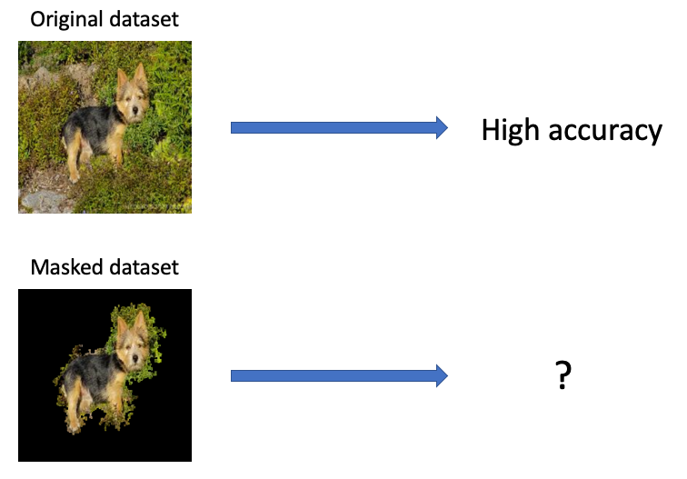
What happens when we mask out the "unimportant" parts of an image?

03 Dec 2019

Japanese below | Comments

In this post, we will experiment and observe how keeping the important regions of an image and masking the rest affects the accuracy of several state-of-the-art convolutional neural networks.

Important pixels and where to find them

Explainability in machine learning is an increasingly popular topic - understanding why certain predictions were made is necessary for humans to trust machine learning models and deploy them in real-life scenarios. Several methods have been proposed already, like LIME (Ribeiro et al., 2016) and KernelSHAP (Lundberg & Lee, 2017), which allow us to understand which parts of an input was important for a particular prediction by assigning attribution scores to feature values. These are model-agnostic methods, meaning that they do not assume anything about the target model’s architecture or parameters (they are treated as black boxes).

Today we will look at a model-specific method, in particular, Integrated Gradients (Sundararajan et al., 2017). This method is focused on neural networks as it relies on being able to evaluate the gradients of the model’s output with respect to the input. The goal of Integrated Gradients is to figure out which pixels in an image contributed most to the neural network’s prediction.

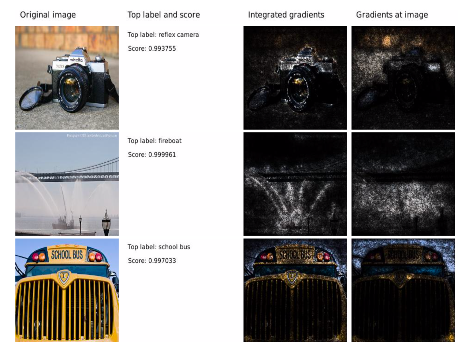
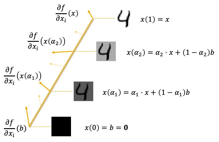
So how does Integrated Gradients work? The method involves taking the input image, the neural network, and some baseline image (e.g. a black image or random noise) to observe how the model’s prediction changes as we linearly interpolate between the baseline and input images. In particular, we measure the gradients at each interval of a linear path between the input and the baseline, then summing the gradients to find the final attributions per pixel. More formally, Integrated Gradients are calculated as follows:

\[\begin{equation*} IntegratedGradients_i(x) = \frac{x_i - b_i}{m} \sum_{h=1}^m \frac{\partial f}{\partial x_i}( b + \frac{h}{m}(x-b) ) \end{equation*}\]

This equation finds the attribution value of each pixel $i$ in the input image $x$. $b$ represents the baseline image, and $m$ is the number of steps between $x$ and $b$, so $b + \frac{h}{m}(x-b)$ is the interpolation between $x$ and $b$ at step $h$ out of $m$. We then get the gradient of the model output $f$ at pixel $x_i$ for this interpolated input ($\frac{\partial f}{\partial x_i}$). Finally we evaluate the weighted sum of the gradients at each interpolation step $h$ to find the Integrated Gradients attribution for each pixel.

Integrated Gradients supports several axioms which are desirable for gradient attribution methods. While we won’t discuss these in detail, here’s a very brief summary of each:

• Sensitivity: if two inputs differ by one pixel and get different predictions, then that pixel should get a non-zero attribution score.
• Implementation invariance: if two models have the same outputs for every input, then Integrated Gradients should produce the same attributions for both models, even if they are implemented differently.
• Completeness: the attribution scores computed by Integrated Gradients should sum to the difference between the prediction of the input image and that of the baseline.

Do checkout their paper and slides for more details! We will now move onto the experiments.

Masking out unimportant parts

Here are the steps we take to mask out an image using integrated gradients:

1. Inputs: an image, a model, cut off percentage $p$
2. Apply Integrated Gradients on the image
3. Create “components” but summing the attribution scores of 3x3 squares
4. Select the top $p \%$ of 3x3 squares based on total attribution scores
5. Set pixels not in top $p \%$ of components (i.e. the unimportant parts) to zero

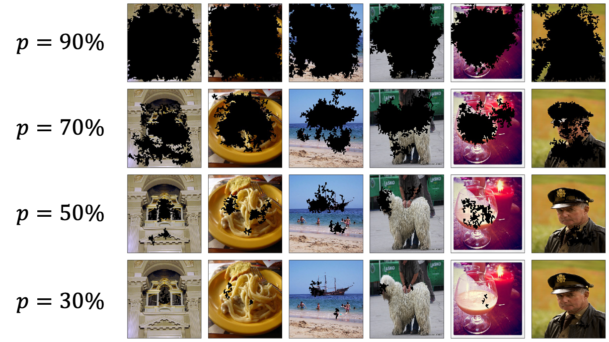
It’s important to note that, taking the top 50% of gradient attributions does not mean taking 50% of all pixels. We rely on the PyTorch implementation found here for computing Integrated Gradients attributions. We apply this procedure to all validation images in ImageNet to create a masked dataset. For $p$, we choose a range of values (90, 70, 50, and 30).

Here are some example images:

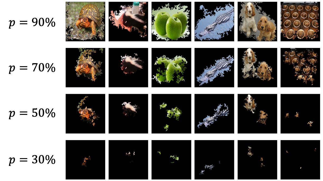
Most images are still recognisable when $p=90$ or $p=70$, whereas the objects are no longer identifiable when $p=30$.

We compare several pre-trained models from PyTorch’s torchvision.models module (documentation). For these experiments, we will just compare the top-1 accuracies of each model on the masked datasets.

Experiments and results

Here are the numbers:

Model	Original Top-1 Accuracy	p=90	p=70	p=50	p=30
VGG-16	71.59	31.79	8.38	0.91	0.17
Inception V3	77.45	50.13	18.89	1.71	0.17
ResNet-50	76.15	46.97	16.66	1.73	0.19
DenseNet-121	74.65	59.21	25.82	2.98	0.26

Accuracy deteriorates as $p$ decreases, and at $p=30$ the models are only slightly better than random guessing. What’s surprising is that, even when we keep the top 90% of gradient attributions and their respective pixels, the models’ accuracies drop significantly (more than half for VGG-16!). The results suggest that these convolutional neural networks require the entirety of the image in order to reach state-of-the-art accuracy, even if we keep the most important features.

This got me thinking of another experiment to further test this hypothesis - what if we deliberately mask out the important regions of an image and test the models’ accuracies? So instead of keep the top 90% of gradient attributions, we keep the bottom 10%. Such a dataset would look like this:

The lower $p$ is, the more visible the images are as we hide fewer pixels. Here are the accuracies of each model:

Model	Original Top-1 Accuracy	p=90	p=70	p=50	p=30
VGG-16	71.59	0.16	2.53	16.06	30.30
Inception V3	77.45	0.15	3.47	23.31	43.97
ResNet-50	76.15	0.14	3.35	22.50	41.83
DenseNet-121	74.65	0.26	5.68	31.55	52.79

As expected, accuracy increases as we decrease $p$. However, when you compare these results to the first table, something weird is apparent. Take a look at $p=50$. For the VGG-16 model, when we keep the top 50% of attributions, we get an accuracy of 0.91%, whereas when we keep the bottom 50% worth of attributions, we instead get 16.06%! Just to check, I compared images which keep the top 50% of gradient attributions to images that keep the bottom 50%. One would assume that the top 50% of gradient attributions and corresponding pixels would yield better visual clues. Well, here’s the comparison:

Model	Top 50% of gradient attributions	Bottom 50% of gradient attributions
VGG-16	0.91	16.06
Inception V3	1.71	23.31
ResNet-50	1.73	22.50
DenseNet-121	2.98	31.55

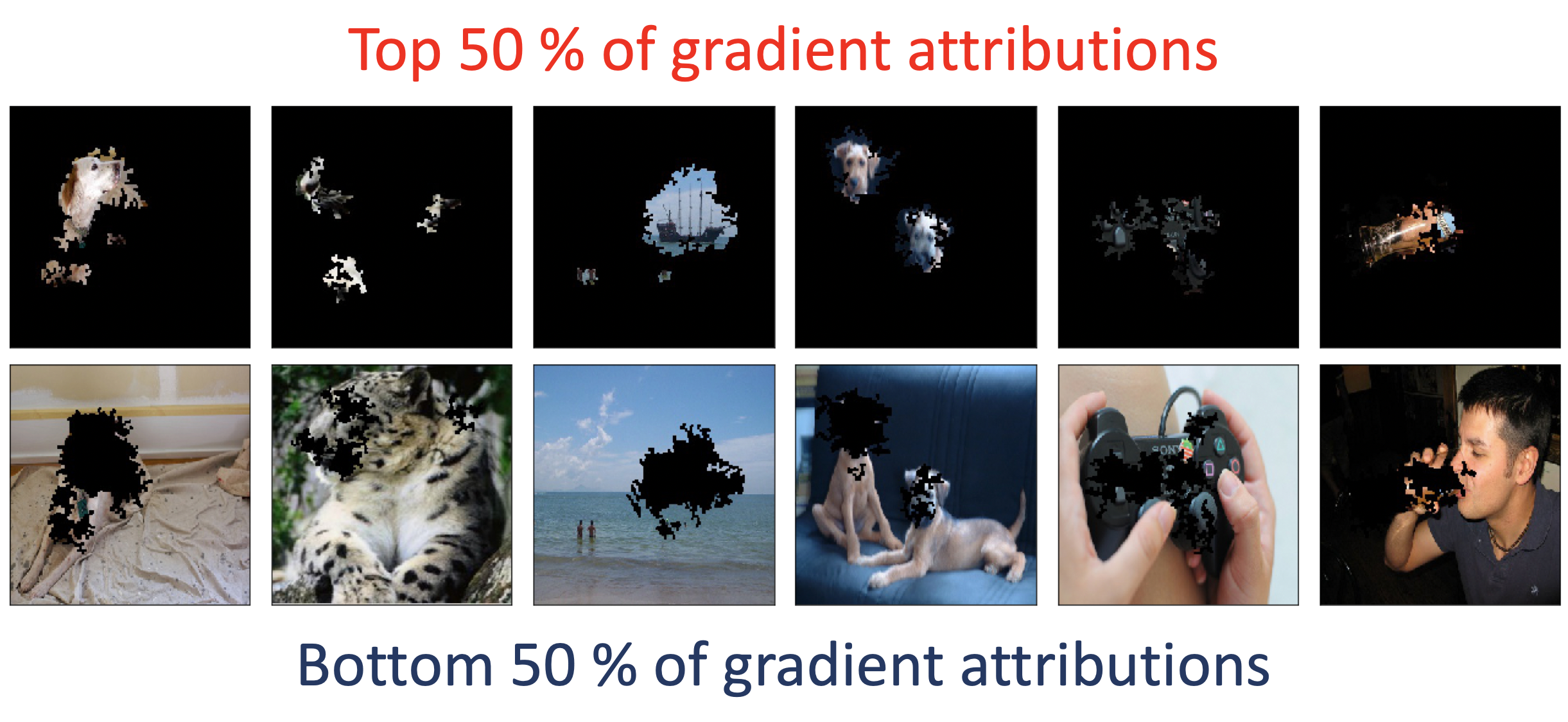
For some images, keeping the top 50% of gradient attributions indeed carves out the object itself (e.g. the medieval ship off the coast in the third image from the left). But it does appear that, for some images, keeping the top 50% removes too much context to the point where it’s even difficult for a human to identify the objects. What do you think? As mentioned earlier, taking the top 50% of gradient attributions does not mean taking 50% of all pixels. Therefore for some images, the top 50% of gradient attributions may correspond to a smaller proportion of pixels.

Summary and thoughts

In this article, we explored Integrated Gradients, a popular way to generate gradient-based attributions for each pixel, and use it to create datasets where we mask out important or unimportant regions of pixels. We then experimented with several state-of-the-art convolutional neural networks and measured their accuracies on these datasets. Interestingly, even when keeping the top 90% of gradient attributions and their corresponding pixels, the top-1 accuracies of these models drop significantly. Perhaps even more surprising is that keeping the bottom 50% of gradient attributions gave higher accuracy than keeping the top 50%.

What conclusions can be made out of these experiments? It’s probably safe to say that state-of-the-art neural networks require the entirety of the input image in order to reach high performance. But these results have in fact raised more questions for me:

• Why do the bottom half of gradient attributions yield higher accuracy than images taking the top half?
• What if we train a model from scratch using one of these masked datasets? Or mix regular images with these masked images? Would this improve model robustness?
• Is there (or should there exist) some correlation between $p$ and overall accuracy of the model? E.g. if I keep the top 90% of gradient attributions should I expect at least 90% of the original accuracy?

These questions would likely lead to separate investigations for the future. Do reach out if you have questions, any ideas about the above questions, or want to collaborate! Please refer to the References for a list of cited papers.

画像の非重要ピクセルをマスキングして生成したデータセットでneural networkの精度を測ってみた

Back to English

今回の記事では、画像の重要ピクセルを探し、それ以外をマスキングした新たな画像データセットに対しての neural networkの精度を測ってみます。

重要ピクセルの求め方

前回の記事 でもテーマとして挙げていましたが、機械学習モデルの挙動を説明・解釈するアルゴリズムの研究・開発 は最近徐々に注目を浴びており、特に機械学習のプロダクト開発においてモデルの信頼度を上げることがより重要になってきています。 最近ではLIME (Ribeiro et al., 2016)やKernelSHAP (Lundberg & Lee, 2017) といったブラックボックス手法（説明対象となるモデルのパラメータやアーキテクチャが不可知的であるという設定） が人気ですが、今回の実験ではIntegrated Gradients (Sundararajan et al., 2017) というmodel-specificな手法を用います。

では、Integrated Gradientsとは何か？上の画像のように、画像の各ピクセルがneural networkの 判断にどれくらい貢献したのかを求める手法です。上記の図では、貢献度が高いピクセルが 明るく表示されており、それ以外は暗くなっています。貢献度の求め方を要約すると、ベースラインとなる画像 （ノイズや真っ黒な画像等）と説明対象の画像の線形補間を行い、各区分においてのneural networkの勾配を求め、 それらの加重和を算出するといった感じです。数式的には以下のようになります。

\[\begin{equation*} IntegratedGradients_i(x) = \frac{x_i - b_i}{m} \sum_{h=1}^m \frac{\partial f}{\partial x_i}( b + \frac{h}{m}(x-b) ) \end{equation*}\]

上記の式は画像$x$の各ピクセル$i$の貢献度を求め方を表しています。$b$がベースライン画像、$m$ が区分数となっており、$b + \frac{h}{m}(x-b)$が$x$と$b$の線形補間になっています。また、この 線形補間においてのneural networkの勾配が$\frac{\partial f}{\partial x_i}$となっており、 これらの加重和を取ることでピクセルの貢献度を算出することができます。

この手法は力学でも使われている 経路積分(path integral)と類似しており、イメージとしてはベースライン画像を始点とし、 対象画像を終点とすると、始点から終点への線形経路を求めるといった感じです。また、LIMEやSHAPとは違い、 Integrated Gradientsはneural networkの勾配を用いて貢献度を測っている為 model-specificな手法として分類されます。

Integrated Gradientsは他の勾配ベースの説明法と比べて幾つかの理論的性質を有しています。 今回は詳しい解説を省きますが、ざっと説明しておきます。

• 感度(Sensitivity): 二つの画像がたった一つのピクセルで違っていて、同じモデルが別々の判断を出したら、 そのピクセルの貢献度はゼロ以外であること（要はそのピクセルの判断のずれへの関与を捉えられること）。
• 実装に対しての不変量性(Implementation Invariance): 二つのモデルが全ての画像において 同じ挙動を表しているのならば、例えそれぞれの実装が違っていても同じ貢献度を算出できること。
• 完全性(Completeness): Integrated Gradientsの和が対象画像とベースライン画像の判断の差に該当すること（i.e. 経路積分と同様な性質)。

詳しくは論文と プレゼン をご参照下さい。続いて実験の解説に移りたいと思います。

非重要ピクセルのマスキング

今回の実験では以下の手順を用いて画像の非重要ピクセルのマスキングを行なっていきます。

1. インプット: 対象画像、モデル、しきい値$p$
2. 対象画像とモデルを基にIntegrated Gradientsを算出する
3. ３x３のピクセル群を構成し、貢献度の和を測る
4. 3.の和を基に上位$p \%$のピクセル群を選択する
5. それ以外の群に属するピクセルをマスキングする

ここではっきりさせたいのが、貢献度上位50%のピクセル数 != 画像ピクセル数の50% ということで、貢献度上位50%のピクセル数が少ないことは有り得ます。 実験の実装は主にPyTorchを用い、Integrated Gradientsの実装はこちらの リポジトリから拝借します。 説明対象画像はImageNetのvalidation imagesとし、上記の手順を適用することで新たなデータセットを 構築します。$p$は90, 70, 50, 30を使います。

上記の手順に従い新たに構築したデータセットは以下のようになります。

$p=90$, $p=70$ではまだ画像の分類が人目でも分かりそうですが、$p=30$の時はほとんど認識不可能 かと思います。

また、説明対象モデルはPyTorchのtorchvision.modelsから幾つか選んで使い、Top-1精度を 比べてみます(詳細)。

検証結果

以下が検証結果です。

Model	Original Top-1 Accuracy	p=90	p=70	p=50	p=30
VGG-16	71.59	31.79	8.38	0.91	0.17
Inception V3	77.45	50.13	18.89	1.71	0.17
ResNet-50	76.15	46.97	16.66	1.73	0.19
DenseNet-121	74.65	59.21	25.82	2.98	0.26

$p$を上げるにつれ精度が下がることが分かります。$p=30$での各モデルの精度はランダムに当てる際の精度と （0.1%)とさほど変わりません。しかし、割と興味深いのは$p=90$の時でも精度がかなり下がるということです。 特にVGG-16の場合は、貢献度上位90%分のピクセル群を残しても精度が半減してしまいます。高い精度を得るには やはり画像全体が必要なのかもしれません。

ついでに非重要ピクセルを残して重要ピクセルを隠すという上記の実験とは逆の設定での検証も行いました。 例えば$p=90 \%$の時、上位90%のピクセル群をマスキングしてデータセットを構築します。以下のように、 $p$が低いほどマスキングしている領域が小さいことが分かります。

そしてこちらがこの新たなデータセットを使って精度を検証した結果です。

Model	Original Top-1 Accuracy	p=90	p=70	p=50	p=30
VGG-16	71.59	0.16	2.53	16.06	30.30
Inception V3	77.45	0.15	3.47	23.31	43.97
ResNet-50	76.15	0.14	3.35	22.50	41.83
DenseNet-121	74.65	0.26	5.68	31.55	52.79

想定内ですが、$p$を下げるほど精度が上がることが分かります。しかし、$p=50$においての重要ピクセルを キープした画像データセットとマスキングした画像データセットの精度を比較してみると、前者が0.91%なのに対し、後者が なんと16.06%なのです。貢献度下位50%のピクセルを残した画像データセットにおいての精度が貢献度上位50%のピクセルを 残したものより遥かに高いのです。念の為、両者の画像を比較してみました。

Model	Top 50% of gradient attributions	Bottom 50% of gradient attributions
VGG-16	0.91	16.06
Inception V3	1.71	23.31
ResNet-50	1.73	22.50
DenseNet-121	2.98	31.55

実際に画像を見てみると、左から三枚目の画像にある船のようにオブジェクト自体が括り抜かれるケースもあれば、 重要ピクセルだけでは認識しづらいものもあることが分かります。逆に重要ピクセルを隠しても認識できる 画像がいくつかあるようです。

まとめ

本記事では、Integrated Gradientsという機械学習説明的モデルを使って画像の重要ピクセルを残した+ 隠した画像データセットを構築してみました。また、それらを使って、幾つかの畳み込みneural networkの 精度を検証してみました。興味深い結果として、貢献度上位90%のピクセルを残した画像データセットでも 精度ががた落ちしたことが挙げられますが、貢献度下位50%のピクセルを残したデータセットの方が上位50%の ピクセルを残したデータセットよりも精度が高いという結果にも驚かされました。

結論として、高い精度を得るにはやはり画像全体が必要だと言えます。同時に新たな疑問も増えました。

• なぜ貢献度下位50%のデータセットの方が上位50%のものより精度が高いのか？
• マスキングした画像データセットを用いてモデルを再学習させたらどうなるのか？
• Integrated Gradientsで得たピクセルごとの貢献度とモデルの精度の関係性はどうあるべきか？例えば貢献度90%分のピクセル を残したら元々の精度の90%くらいの精度を期待するべきか？

等々、色々と実験する余地が有りそうです。

以上となります。質問やコメントのある方は是非ご連絡ください。最後まで読んで頂き有難うございました！

References

1. Ribeiro, M. T., Singh, S., & Guestrin, C. (2016). "Why Should I Trust You?": Explaining the Predictions of Any Classifier. Proceedings of the 22nd ACM SIGKDD International Conference On Knowledge Discovery and Data Mining, San Francisco, CA, USA, August 13-17, 2016, 1135–1144.
2. Lundberg, S. M., & Lee, S.-I. (2017). A Unified Approach to Interpreting Model Predictions. In I. Guyon, U. V. Luxburg, S. Bengio, H. Wallach, R. Fergus, S. Vishwanathan, & R. Garnett (Eds.), Advances in Neural Information Processing Systems 30 (pp. 4765–4774). Curran Associates, Inc. http://papers.nips.cc/paper/7062-a-unified-approach-to-interpreting-model-predictions.pdf
3. Sundararajan, M., Taly, A., & Yan, Q. (2017). Axiomatic attribution for deep networks. Proceedings of the 34th International Conference on Machine Learning-Volume 70, 3319–3328.