Explaining Away Attacks Against Neural Networks

Japanese below | Acknowledgements | Comments

In this article, we will demonstrate how to fool a neural network into predicting an image of an elephant as a ping-pong ball. We will also see whether we can defend against such attacks by explaining the model’s decisions. Code for this blog post can be found here. You can also checkout the poster I created based on this project here.

The surprising brittleness of neural networks

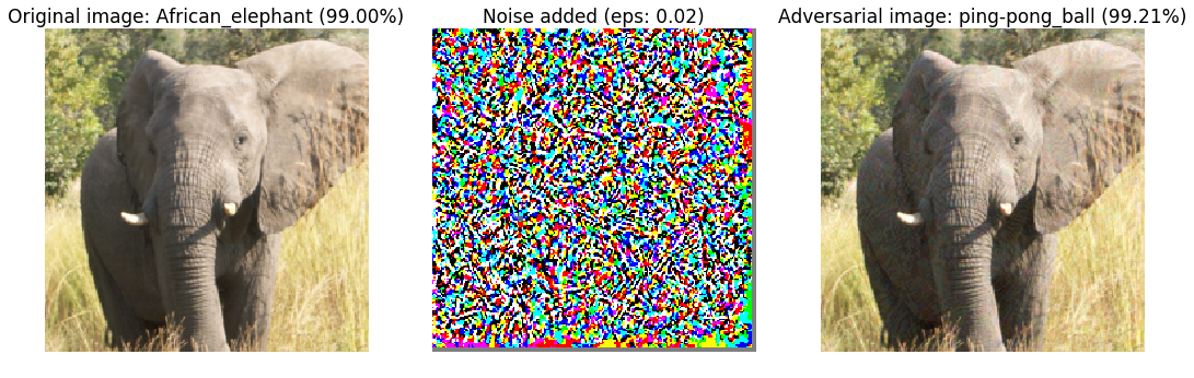
The image you see above is the result of an adversarial attack towards an Inception V3 model (Szegedy et al., 2016), a popular and powerful neural network that produced impressive results on image classification datasets some years ago. As the name suggests, the goal of an adversarial attack is to attack a neural network and cause unintended behaviour. The image on the far left is the “ordinary image” which a neural network correctly classifies as an African elephant with 99% confidence. The image on the right is obtained by adding the image on the left with the noisy image (middle). The resulting “perturbed image” still looks like an African elephant, but this time the same network predicts “ping-pong ball” with even higher confidence.

Even though neural networks are producing outstanding results across many tasks, we’re also starting to discover several surprising shortcomings like the one above. The field which studies such vulnerabilities is called adversarial machine learning.

Key concepts

As an introduction to the field, here are some of the key concepts in adversarial machine learning:

• An adversarial example is an input that is perturbed to cause misbehavior from a target model
• A white-box attack is an attack where the assailant has knowledge of the target model’s details, including its parameters, output, and architecture.
• A black-box attack, on the other hand, is an attack where the assailant only has query-access to the model, and does not know its parameters. As one can imagine, black-box settings are more realistic in practice.
• A targeted attack is an attack where the assailant tries to solicit some desired behavior from the target model. In the case of classification problems, this translates to causing the model to predict a particular class.
• On the other hand, in a untargeted attack, the assailant simply wishes to cause the model to predict something incorrect.

The Fast Gradient Sign Method (FGSM)

Numerous ways to attack neural networks already exist. One of the earliest methods is called the Fast Gradient Sign Method (Goodfellow et al., 2014). The core concept of the untargeted version of the attack is simple - neural networks are trained to minimize some loss function, so why not perturb the input image in the direction which increases this loss function? This is equivalent to gradient ascent, where we are leading the neural network’s prediction away from the correct class. Formally, an untargeted FGSM attack finds the following following:

where $J(x, y)$ is the loss function of the model, $\nabla_x J$ is the gradient of the loss function with respect to the input (instead of the weights of the model as is done in backpropagation), $ \epsilon$ is some scalar parameter which controls the magnitude of the perturbation added to input $x$ to generate adversarial example $\tilde{x}$. $y$ refers to the groundtruth of $x$.

In the targeted setting, the assailant chooses some target class $y_t$ so that the model outputs the desired prediction. So instead of gradient ascent with the correct class $y$ as was done with the untargeted attack, targeted FGSM does gradient descent with $y_t$. In other words, we perturb the input in the direction that minimizes the distance between the network’s prediction and $y_t$:

As the equations suggest, FGSM only requires one step of gradient ascent/descent. Hence it is also commonly referred to as a single-step gradient attack. There is also an iterative variant of FGSM, or the Basic Iterative Method (BIM) (Kurakin et al., 2016):

which is a strictly more effective attack compared to FGSM. In our experiments below, we will be using BIM to generate more effective adversarial examples. First, we implement the FGSM attack below using pytorch:

def fgsm_attack(image, epsilon, data_grad, targeted=False):
    direction = -1 if targeted else 1    

    # Collect the element-wise sign of the data gradient
    sign_data_grad = data_grad.sign()

    # Create the perturbed image by adjusting each pixel of the input image
    perturbed_image = image + direction*epsilon*sign_data_grad

    # Adding clipping to maintain [0,1] range
    perturbed_image = torch.clamp(perturbed_image, 0, 1)

    return perturbed_image

The fgsm_attack function takes four parameters - image, which is the image which will be perturbed, epsilon, which controls the level of noise added to image, data_grad, which are the gradients of the loss function with respect to the inputs, and targeted, a boolean telling the function whether the attack is an untargeted or targeted one. To turn this attack into an iterative one, we simply run FGSM a specified number of iterations:

data.requires_grad = True

for i in range(num_iterations):
    output = F.log_softmax(model(perturbed_data), dim=1)

    # Calculate the loss
    loss = F.nll_loss(output, target)

    # Zero all existing gradients
    model.zero_grad()

    # Calculate gradients of model in backward pass
    loss.backward()

    # Collect datagrad
    data_grad = data.grad.data

    # Call FGSM Attack
    perturbed_data = fgsm_attack(data, epsilon, data_grad, targeted=True)

F.log_softmax is the activation function applied to model(perturbed_data), which returns the logits (pre-activation output) of the neural network. According to PyTorch’s documentation, the F.nll_loss we use for calculating the loss and subsequently the gradient for perturbation expects log-scaled outputs, which is why we use log_softmax instead of regular softmax.

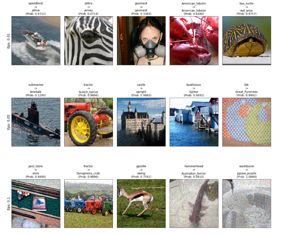
The grid of images above (best seen in a large screen) shows additional examples of targeted iterative FGSM attacks. You will observe how increasing epsilon also causes more visible perturbations to the images but also increases the efficacy of the attacks.

While we have focused on images so far, adversarial attacks have also been proposed for NLP, audio, and reinforcement learning models. It seems that any neural network is vulnerable to adversarial attacks.

Explaining neural network predictions

As a final prelude to the main topic of the blog post - explaining a neural network’s output on an adversarially perturbed image - I would like to discuss what it actually means to explain the output of some machine learning model.

Explaining via feature attributions

So far in academia, one of the most common approaches towards explaining the prediction of a machine learning model is to assign scores to each portion of an input, where the score reflects how much that portion of the input contributed to the model’s decision. This is also called additive feature attribution. More formally, an explanation is a linear function $g$:

where $x_i’$ is a binary variable that represents the original input feature $x_i$, $\phi_i$ represents the contribution of each feature, and $M$ is the number of binary variables. $g(x’)$ is the explainer model that is parameterized by the $\phi$s. Hence The expression $\phi_ix_i$ denotes how much a particular interpretable feature is contributing to the model’s prediction when $x_i’=1$. In other words, the parameters of $g$ represent the explanation itself. The higher $\phi_ix_i$ is the more $x_i$ has contributed to the original prediction.

The binary variables $x_i’$s are also called the interpretable representations of $x_i$ and help make explanations more intuitive and understandable to us humans. In short, interpretable representations rely on the segmentation of inputs. We typically look at individual pixels or patches of pixels (also called superpixels) for images and individual tokens for text data (i.e. Bag-of-Words).

How does the explanation model $g$ learn the attribution scores $(\phi_1, \dots \phi_M)$? There exist several approaches, but we will discuss the one taken by LIME (Locally Interpretable Model-agnostic Explanations) (Ribeiro et al., 2016). Denoting the model to be explained as $f$, the key intuition is that we would like to train $g$ such that its predictions match those of $f$. In other words, we would like to achieve $f(x) = g(x’)$. Training data for $g$ is generated by perturbing $x’$ to obtain additional interpretable inputs $z’$. According to the LIME paper, this perturbation is done by randomly flipping 1’s in $x’$ (which, remember, is just a binary vector) to 0’s. For text data, for example, this is equivalent to removing individual tokens from the document. The perturbed interpretable input $z’$ is then converted to its original input representation $z$, which is then used to obtain $f(z)$. Making many pairs of $z’, f(z)$ creates a suitable dataset to train $g$ with.

It is worth noting that, because we only have query access to $f$ in generating training data, we don’t need to know the model’s parameters or specifications. This is where LIME’s model-agnosticism comes from. Finally, $g$ is trained by minimizing the following:

Here, $L$ is called the faithfulness loss, which is simply the distance between $g(x’)$ and $f(x)$, which is weighted by another distance measure $\pi_{x}$. In practice, we calculate the squared difference between $f$ and $g$, and $\pi$ is a Gaussian distribution around $x$. Intuitively speaking $\pi$ allows the model to focus on perturbed samples $z’$ which are closer to $x’$:

Finally, $\Omega$ represents the complexity of $g$. Minimizing the complexity of the explanation is necessary for it to be simple and intuitive, which are desired qualities of an explanation. Since $g$ is a linear model, the complexity of $g$ is defined as the number of non-zero weights. In other words, the number of non-zero $\phi$s represents the number of features that explain a particular prediction. In practice, this is achieved by applying LASSO regularization when training $g$.

The SHAP framework

While LIME gives good intuition on how a explanation model is formulated and trained, we will be using another framework for our ensuring experiments called SHAP (SHapley Additive exPlanations) (Lundberg & Lee, 2017), which was published in NeurIPS 2017 under the title: “A Unified Approach to Interpreting Model Predictions”.

As the title suggests, SHAP is a framework that builds upon various prior works for explainability such as LIME and DeepLIFT (Shrikumar et al., 2017). SHAP also relies on additive feature attribution; in particular, it applies concepts from cooperative game theory to existing frameworks in order to obtain special attribution scores called SHAP values, which satisfy a set of desirable theoretical properties (you can find more details from the original paper).

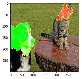
For image-based explanations, SHAP wraps another attribution method called Integrated Gradients (Sundararajan et al., 2017). In short, the method measures the cumulative change in gradients in a neural network by comparing the input image to a baseline (i.e. a blank image) while satisfying several theoretical qualities. The resulting explanation is a heat map over the input image, where each pixel is assigned an attribution score. The following code and image (taken directly from the SHAP tutorial) is an example of applying SHAP and Integrated Gradients to a pre-trained PyTorch model:

import torch, torchvision
from torch import nn
from torchvision import transforms, models, datasets
import shap
import json
import numpy as np

# load the model
model = models.vgg16(pretrained=True).eval()

X,y = shap.datasets.imagenet50()

X /= 255

to_explain = X[[39, 41]]

# load the ImageNet class names
url = "https://s3.amazonaws.com/deep-learning-models/image-models/imagenet_class_index.json"
fname = shap.datasets.cache(url)
with open(fname) as f:
    class_names = json.load(f)

e = shap.GradientExplainer((model, model.features[7]), normalize(X))
shap_values,indexes = e.shap_values(normalize(to_explain), ranked_outputs=2, nsamples=200)

# get the names for the classes
index_names = np.vectorize(lambda x: class_names[str(x)][1])(indexes)

# plot the explanations
shap_values = [np.swapaxes(np.swapaxes(s, 2, 3), 1, -1) for s in shap_values]

shap.image_plot(shap_values, to_explain, index_names)

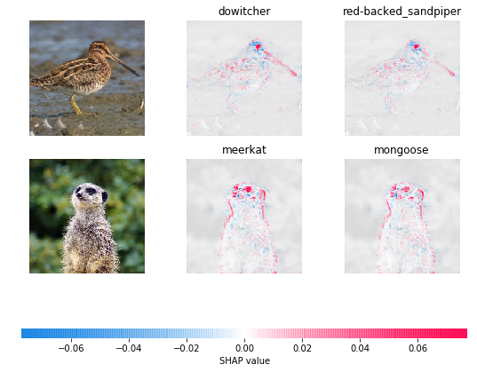
The red regions above represent positive SHAP values, or pixels that support the class predicted by the model, whereas the blue regions represent negative SHAP values which are evidence against the predicted class. Qualitatively speaking, one can see how the relevant features of each image are assigned high positive scores.

Can we “explain away” adversarial examples?

As we just saw, SHAP allows us to see how much each pixel contributes to the neural network’s prediction. We finally can address our original question - what happens when we apply SHAP to adversarially perturbed images? Again, we use the GradientExplainer module in SHAP to measure gradient activations for each pixel:

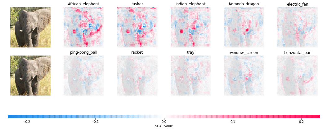
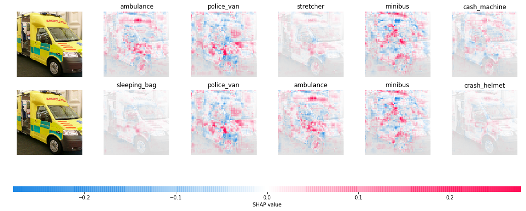
The above image juxtaposes the explanations for a clean image (above) and its adversarial counterpart (below). You will immediately notice that there is a significant discrepancy in the activations for clean image as opposed to perturbed image - SHAP values for the “correct” class are much sharper compared to those for the targeted class. Here are a few more examples below:

Ambulance vs. sleeping bag

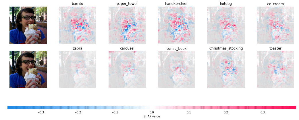
Burrito vs. zebra

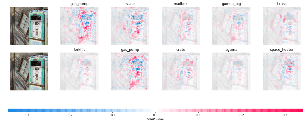
Gas pump vs. forklift

It seems that the SHAP values are consistently higher for the correct class. In comparison, the SHAP values for the targeted class are much smaller. This is despite the fact that the model’s output probabilities for the targeted classes are very high (~99%)! The histogram below represents a statistical comparison of the average SHAP values for the top prediction of clean and adversarial images using 1000 ImageNet test images:

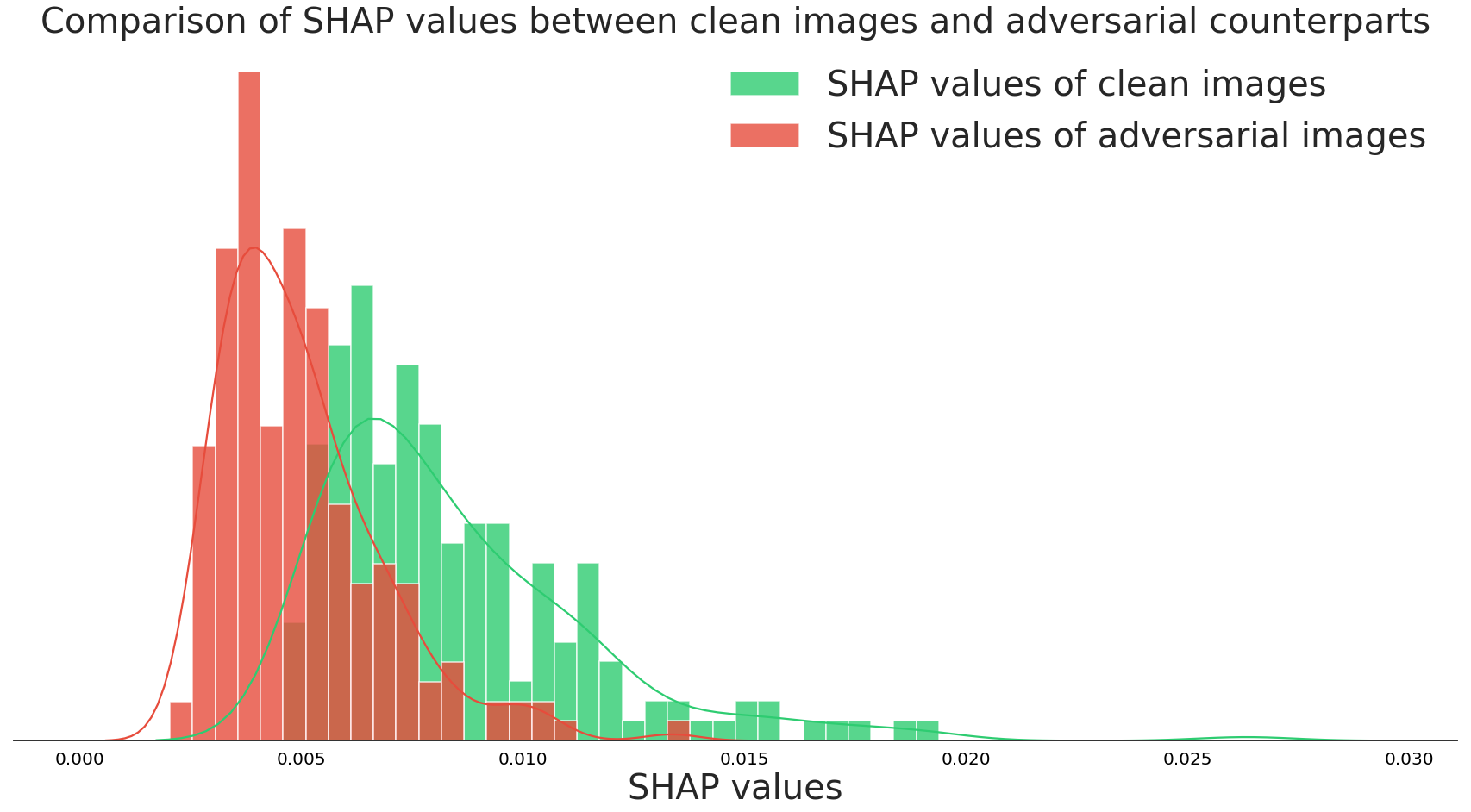
What do these results suggest? It appears that, while we cannot detect adversarial examples with our eyes, we can use SHAP and a model’s predictions to determine whether a given prediction “makes sense.” In other words, if there is insufficient evidence for a particular prediction then there is a higher chance for the input to be adversarial. It then makes sense to use a framework like SHAP since it is able to ascertain the average prediction of the classifier. A burrito looks very different from an average zebra - hence there’s little evidence in the form of gradient activations.

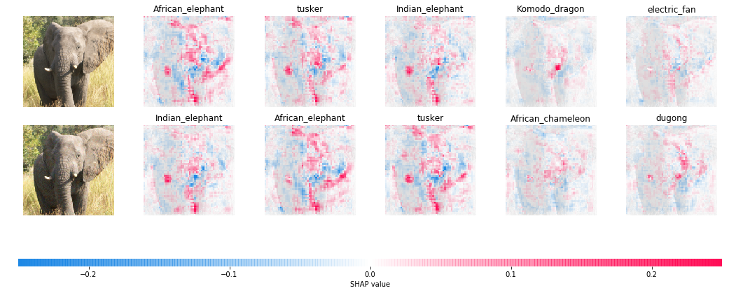
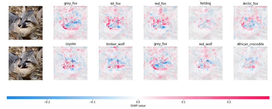
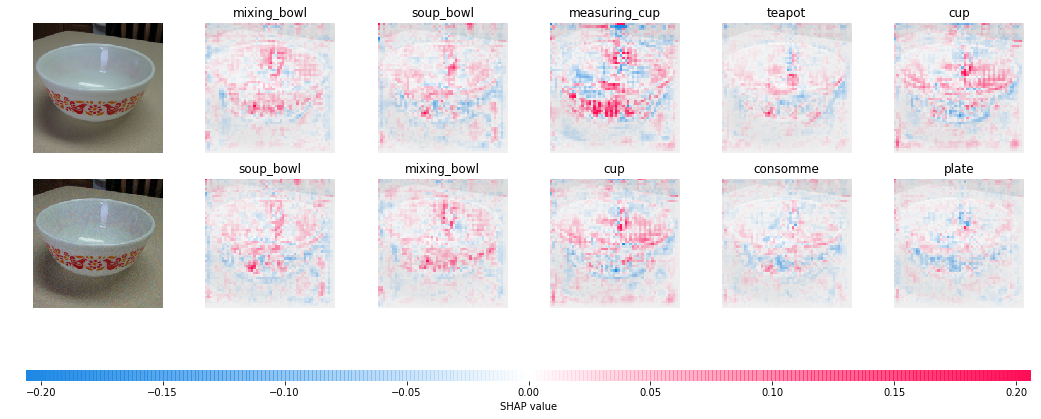
Of course, this is not a silver bullet in terms of defending against adversarial attacks. Our experiments have so far dealt with adversarial examples where the target classes were chosen randomly. What happens if we target semantically similar classes?

African elephant vs. Indian elephant

Grey fox vs. coyote

Mixing bowl vs. soup bowl

Moving van vs. minivan

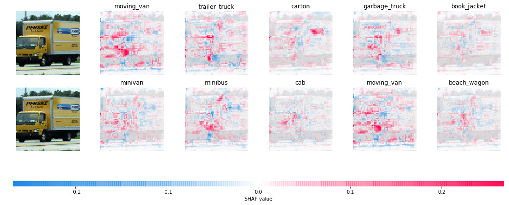
It seems that our “defense” becomes a lot less effective. Intuitively, an African elephant looks similar to an Indian elephant and hence the evidence for one class would also support a prediction for the other. While SHAP cannot “explain away” difficult adversarial examples like these, our experiments above reveal the potential of using frameworks for explainability to make neural networks more robust and reliable.

Summary

In this blog post we covered the following topics:

• The brittleness of neural networks and attacking them with methods like FGSM
• Explaining the predictions of neural networks
• Using SHAP and Integrated Gradients to “explain away” easy adversarial examples

Moreover, these experiments shed light on an apparent disconnect between a neural network’s confidence and the evidence that it provides. That is, even if a neural network is highly confident about its prediction, it may not necessarily provide enough evidence. This is especially important to consider when neural networks are deployed in real-life scenarios where users must take action based on a model’s output. Making machine learning models more reliable is necessary if they are to be deployed successfully in real-life scenarios.

With that we come to the end of the English section of this blog post. Thanks for sticking around! Do checkout the References section for the list of academic works I’ve cited. If you have any questions or feedback, feel free to reach out!

Neural networkの判断根拠を用いた攻撃への防御

Back to English

Neural networkと言えば、画像認識や、自然言語処理、音声認識等といった様々な分野で大きな 成果を出している最先端の機械学習モデルです。最新の論文や機械学習系のスタートアップでもneural networkは 幅広く利用されています。しかし、そんな高性能のモデルでも最近では大きな脆弱性が発見されていることはご存知でしょうか？ 実はneural networkは誤った判断をさせることが容易にできます。今回の記事では、 この特異な脆弱性について話しながら、neural networkの判断を解釈することでその脆弱性を解消できるかを検証してみます。

Neural networkの脆弱性

上にある左側の画像は、ImageNetというデータセットからとったアフリカゾウの一画像で、学習済みの Inception V3 (Szegedy et al., 2016) というneural networkを用いると99%の信頼度で「アフリカゾウ」に正しく分類されます。 この画像に中央の「ノイズ」を加えることで右側の画像を得ることができますが、 見ての通り、オリジナルの画像との区別が付きません。しかし、同モデルで右側の画像を分類してみると今度は 99.21%の信頼度で「ピンポン玉」という予測が出ます。 このような、人の目では判別できないような変化を 元の画像に加えることによってneural networkに誤った判断をさせる行為を adversarial attack といい、 こういった現象を研究する分野を adversarial machine learning と呼びます。

用語

以下にadversarial machine learningの主な用語を説明していきます。

• Adversarial example: neural networkに誤った判断をさせる為に人為的に作られたインプット
• White-box attack: 攻撃者が、ターゲットのneural networkのパラメータやアーキテクチャ、 そして判断等の情報を有していて、それらを利用した攻撃のこと
• Black-box attack: White-box attackとは違い、neural networkの判断しか利用できない 攻撃のこと
• Targeted attack: ターゲットのneural networkにAdversarial exampleを予め選択したラベル として分類させることを目標とした攻撃（選択的攻撃）
• Untargeted attack: 選択的攻撃とは違い、分類を問わずただ誤った判断をさせることを 意図した攻撃（無選択的攻撃）

Fast Gradient Sign 手法 (FGSM)

Adversarial machine learningが分野として確立されてから様々な攻撃の手法が提案されてきていますが、 今回の記事では最も代表的な手法の一つであるFast Gradient Sign 手法 (Goodfellow et al., 2014)を紹介していきます。ざっと説明すると、 neural networkの学習の際に最小化されるコスト関数が逆に大きくなる方向を定め、元の画像に適度の ノイズを加えるといった仕組みです。言い換えれば、neural networkの学習に用いるのが勾配降下法なら、 adversarial exampleの生成には勾配上昇法が用いられます。無選択的攻撃は数式的には以下のように表されます。

上記の数式では、$J(x, y)$がコスト関数、$\nabla_x J$が$x$を基にしたコスト関数の勾配、 $\epsilon$がノイズの最大値を設定するパラメータ、$\tilde{x}$がadversarial example、そして $y$が正解値となっています。この手法ではneural networkの判断だけでなく、勾配上昇法に用いられる モデルのパラメータ等も必要なのでwhite-box attackの類に入ります。

選択的攻撃の場合、攻撃者は予めにターゲットのneural networkにアウトプットして欲しいラベル$y_t$ を用意します。無選択的攻撃では勾配上昇法が用いられる一方、選択的攻撃では学習時と同じく 勾配下降法を利用します。即ちモデルの判断が$y_t$に近くなるようにノイズを生成する仕組みです。

FGSMでは、勾配上昇・降下が一回だけ行われます。したがってこのような手法を single-step gradient attack と呼ぶことがあります。これを何回か行ったものを Basic Iterative Method (BIM) (Kurakin et al., 2016) と呼び、 以下のようにadversarial exampleが生成されます。

勾配上昇・降下を何回も行うことによってFGSMよりも効果的なadversarial exampleを生成することが BIMのメリットです。以下ではpythonとpytorchを使って実際にFGSMを実装してみたいと思います。

def fgsm_attack(image, epsilon, data_grad, targeted=False):
    direction = -1 if targeted else 1    

    # 勾配の符号を抽出（1 or -1)
    sign_data_grad = data_grad.sign()

    # 元画像にノイズを加える
    perturbed_image = image + direction*epsilon*sign_data_grad

    # Adversarial imageを[0,1]間にclipする
    perturbed_image = torch.clamp(perturbed_image, 0, 1)

    return perturbed_image

FGSMのパラメータは以下の通りです。

• image: adversarial example生成の対象となる画像
• epsilon: 元画像に加えるノイズの最大値
• data_grad: ロス関数の勾配
• targeted: untargeted或いはtargeted attackを指定するためのフラグ：

Basic Iterative MethodではFGSMを何回か適用します。

data.requires_grad = True

for i in range(num_iterations):
    output = F.log_softmax(model(perturbed_data), dim=1)

    # ロス関数
    loss = F.nll_loss(output, target)

    # 勾配のリセット
    model.zero_grad()

    # 新たに勾配を算出
    loss.backward()

    # データを基にした勾配を抽出
    data_grad = data.grad.data

    # FGSMの適用
    perturbed_data = fgsm_attack(data, epsilon, data_grad, targeted=True)

model(perturbed_data)はモデルのロジットを算出する関数です。また、 PyTorchでは対数のインプット を要する陰性尤度ロス関数のF.nll_lossが使われるので、普通のsoftmax活性関数ではなくF.log_softmax をmodel(perturbed_data)に適用します。

上記のグリッドはBIMを使い生成したadversarial exampleの例です。epsilonを上げることで ノイズがより顕著になることが分かります。

Adversarial attackは画像データに適用されることが多いですが、言語データ、 音声データ、強化学習データにも適用した研究結果もあり、neural networkの脆弱性は データの属性を問わないことが言えます。

Neural networkの判断解釈

さて、今回の記事の本題が「Neural networkの判断解釈を用いた攻撃への防御」となっていますが、 最後の前置きとしてneural networkの判断解釈(英語では explainability)について解説して いきたいと思います。

特徴の帰属による判断解釈

Neural networkは高性能である一方、いかにして判断を下したのかを求めるのが困難です。 したがって最近ではneural network等の複雑な機械学習モデルの判断を解釈することが研究の課題と なっており、neural networkを実世界で利用する産業界でも大きな注目を浴びています。 ではneural networkの判断の解釈とは一体どういうことでしょうか？ 最近の研究ではデータの特徴にスコアを帰属することによってneural networkの判断を解釈しています。 言い換えれば、どの特徴がどれくらいモデルの判断に関与しているかを求めます。英語ではこの手法を additive feature attribution と呼び、数式的には

と表されます。$g(x’)$は判断解釈を算出するモデルで、各$\phi_i$が$g$のパラメータとなります。 元データを$x$とすると、$x’$は$x$を二進法で表したものになり、英語ではこれを interpretable representation と呼びます。即ち$\phi_ix_i’$は$x_i’$が1であるときの neural networkの判断への貢献度を測ります。

このinterpretable representationは主にデータを二進法で表せるように区分したものを指します。 例えば画像データでは各ピクセル或いはピクセルの集合(a.k.a. super pixels)、 言語データにおいては各単語の有無を表す Bag-of-Words 等を用いたりします。

判断解釈モデル$g$はいかにして帰属スコア$(\phi_1, \dots \phi_M)$を学ぶのでしょうか？手法はいくつかありますが、 中でも有名な LIME (Locally Interpretable Model-agnostic Explanations) (Ribeiro et al., 2016)　というモデルに着目してみましょう。ざっと説明すると、 人にとって解釈しやすいシンプルなモデルを、解釈の対象となる複雑なモデルに局所的に近似させるといった手法です。 解釈対象のモデルを$f$とし、解釈モデルを$g$とすると、$f(x)=g(x’)$ になるように$\phi$を最適化することがLIMEの目的です。 機械学習的に$\phi$を最適化するには当然データとラベルが必要ですが、$z’$という、バイナリベクトルである$x’$の1を 幾つかランダムに0にセットしたデータを何個かサンプリングし、それを基に$(z, f(z))$のデータ・正解値ペアを 用意することでデータセットを構築するができます。このデータセットは$x$の周辺に置ける$f$の挙動を 表しており、これを基に$\phi$を最適化することによって$g$を居所的に$f$に近似させることができます。

なお、LIMEの model agnosticism は$f$にはquery-accessしかないという仮定からきています。 即ち論理的にはLIMEはどんな機械学習モデルにも適用できるということです。実際にneural network以外にも XGBoostや他の決定木モデルにも適用されたりできるようなので便利です。さて、LIMEモデルのパラメータは 以下のように最適化されます:

$L$は$f(x)$と$g(x’)$の距離を表すロス関数で、英語では faithfulness loss と呼びます。 またロス関数は$\pi_{x}$という関数で重みをつけています。この$\pi_x$は基本的には正規分布を用いていて、 $z$と$x$の距離を表しています。要するには$z$が$x$に近いほど$f$と$g$の距離が重要視されるということです。 数式的には

と表されます。$\Omega$は$g$の複雑度(complexity)です。モデルの判断解釈は できるだけシンプルで明解なものが好まれるので解釈モデルの複雑度もなるべく抑えたいとのことです。 $g$が線形モデルの場合、重みの数=判断解釈に用いられる 特徴の数なので、0じゃない重みの数を複雑度として測ることができます。LIMEでは判断解釈に要する特徴の数を $k$とすると、K-Lassoという最小二乗法を用いて最適解を得られる$k$個の重みを学習します。

SHAP手法

LIMEの他にもSHAP (SHapley Additive exPlanations) (Lundberg & Lee, 2017)というフレームワークがあります。NeurIPS 2017 で発表された手法ですが、LIMEを含め幾つかの判断解釈法をまとめたことで注目を浴びています。詳しくいうと、 シャープレイ値というゲーム理論の利得分配法を用いたadditive feature attributionの帰属スコアの 算出法を他の判断解釈手法に適用するといったアイデアです。 他の判断解釈法と比べると、シャープレイ値はいくつかの論理的な性質を持っていてより正確な判断解釈を 求めることができるとのことです （論文はこちら）。

SHAPの画像データの判断解釈にはIntegrated Gradients (Sundararajan et al., 2017)という手法がベースになります。 短く説明すると、判断解釈対象の画像データを何らかのベースライン（真黒な画像等）と対比し、neural networkの それぞれの画像で得られる勾配の差を集約したものを元画像にヒートマップとして表すといった手法です。 即ち画像の各ピクセルがどれだけ判断に寄与したかを見ることができます。以下のコードはSHAPの チュートリアル から抜粋したもので、Integrated GradientsをPyTorchモデルに適用し判断解釈をヒートマップとして 生成しています。

import torch, torchvision
from torch import nn
from torchvision import transforms, models, datasets
import shap
import json
import numpy as np

# load the model
model = models.vgg16(pretrained=True).eval()

X,y = shap.datasets.imagenet50()

X /= 255

to_explain = X[[39, 41]]

# load the ImageNet class names
url = "https://s3.amazonaws.com/deep-learning-models/image-models/imagenet_class_index.json"
fname = shap.datasets.cache(url)
with open(fname) as f:
    class_names = json.load(f)

e = shap.GradientExplainer((model, model.features[7]), normalize(X))
shap_values,indexes = e.shap_values(normalize(to_explain), ranked_outputs=2, nsamples=200)

# get the names for the classes
index_names = np.vectorize(lambda x: class_names[str(x)][1])(indexes)

# plot the explanations
shap_values = [np.swapaxes(np.swapaxes(s, 2, 3), 1, -1) for s in shap_values]

shap.image_plot(shap_values, to_explain, index_names)

上の画像の赤い部分が正のシャープレイ値で、モデルの判断を裏付ける根拠として解釈できます。 逆に青いピクセルが負の値を表しており、判断へ相反している部分だと解釈できます。画像のどの部分が モデルの判断に寄与しているのかが大体分かります。

判断解釈で攻撃を防げるか検証してみた

さて、ようやく今回の記事の本題に辿り着くことができました。上のように、SHAPで画像のどの部分が判断に 繋がっているかを算出することができますが、この手法をadversarial exampleに適用するとどうなるか 見てみましょう。上と同じくSHAPのGradientExplainerを使います。

上の列が元画像、下の列がadversarial exampleを利用し左から信頼度の高い順でモデルの分類に対して 算出したシャープレイ値です。元画像に対してのモデルの「アフリカゾウ」という分類には大きなシャープレイ値が見られますが、 すぐ下のadversarial exampleに対する「ピンポン玉」という分類のシャープレイ値のほとんどがゼロに近いです。 同じ99%の信頼度での分類ですが、シャープレイ値には大きな差が見られます。他にもいくつかの画像を対比しました。

救急車 vs. 寝袋

ブリトー vs. シマウマ

ガソリンスタンド vs. フォーク車

他の対比でも元画像のシャープレイ値がadversarial exampleの値より大きいことが分かるかと思います。 分布的にも違いが大体分かります。下記のグラフでは、元画像（緑）及びadversarial example (赤)の 各画像で得られた分類の平均シャープレイ値の分布を表しています。

したがって、元画像とノイズを加えた画像の区別がつかなくても、シャープレイ値が 低いほどadversarialである可能性が高くなると捉えることができます。 そもそもゾウを「ピンポン玉」として分類する根拠が無いのでこの結果は必然的かもしれません。

でもこの手法を使えばどんな攻撃も防げることは残念ながらできないようです。今までは選択的攻撃のラベルを ランダムに採択していましたが、画像の本来のラベルに近いものを利用するとこうなります。

アフリカゾウ vs. インドゾウ

キツネ vs. コヨーテ

サラダボウル vs. お椀

引越しトラック vs. ミニバン

アフリカゾウはインドゾウに視覚的に似ているので、シャープレイ値も当然似てきます。 他の対比の例でもシャープレイ値が似ていることが分かります。

まとめ

最後になりますが、今回の記事では以下のテーマを取り上げました。

• Neural networkの脆弱性とFast Gradient Sign手法(FGSM)等を利用したadversarial exampleの生成
• 機械学習モデルの判断解釈の算出
• SHAPで算出した判断解釈を用いた脆弱性の解消の検証

また、今回はモデルへの攻撃を防ぐという趣旨の記事でしたが、neural networkの判断の信頼度とSHAPで求めた 判断解釈の関係についても一言言えるかと思います。例え判断の信頼度が高くても、それを裏付ける根拠がある という保証はないと今回の実験で分かりました。こういったブレはneural networkの 実世界での利用の障壁になるので、モデルの信頼性を上げるための研究の発展が必要だと思います。

以上となります。初めての記事で色々と改善できる部分も多いと思いますが、内容が読者にとって 面白いものであったならば幸いです。最後まで読んで頂き有難うございました！

Acknowledgements

Many thanks to my friends and colleagues - Aaron, Auguste, Crystal, David, Eugene, Kai, Marco, and Rocco - for providing feedback on initial drafts and providing insightful discussions! And a big thank you to my mother and brother for their unwavering support. This is my first long blog post, and I’m looking forward to writing more.

References

1. Szegedy, C., Vanhoucke, V., Ioffe, S., Shlens, J., & Wojna, Z. (2016). Rethinking the inception architecture for computer vision. Proceedings of the IEEE Conference on Computer Vision and Pattern Recognition, 2818–2826.
2. Goodfellow, I. J., Shlens, J., & Szegedy, C. (2014). Explaining and harnessing adversarial examples. ArXiv Preprint ArXiv:1412.6572.
3. Kurakin, A., Goodfellow, I., & Bengio, S. (2016). Adversarial machine learning at scale. ArXiv Preprint ArXiv:1611.01236.
4. Ribeiro, M. T., Singh, S., & Guestrin, C. (2016). "Why Should I Trust You?": Explaining the Predictions of Any Classifier. Proceedings of the 22nd ACM SIGKDD International Conference On Knowledge Discovery and Data Mining, San Francisco, CA, USA, August 13-17, 2016, 1135–1144.
5. Lundberg, S. M., & Lee, S.-I. (2017). A Unified Approach to Interpreting Model Predictions. In I. Guyon, U. V. Luxburg, S. Bengio, H. Wallach, R. Fergus, S. Vishwanathan, & R. Garnett (Eds.), Advances in Neural Information Processing Systems 30 (pp. 4765–4774). Curran Associates, Inc. http://papers.nips.cc/paper/7062-a-unified-approach-to-interpreting-model-predictions.pdf
6. Shrikumar, A., Greenside, P., & Kundaje, A. (2017). Learning important features through propagating activation differences. Proceedings of the 34th International Conference on Machine Learning-Volume 70, 3145–3153.
7. Sundararajan, M., Taly, A., & Yan, Q. (2017). Axiomatic attribution for deep networks. Proceedings of the 34th International Conference on Machine Learning-Volume 70, 3319–3328.