
Predicting football outcomes with PyStan
27 May 2021We play around with PyStan, a state-of-the-art probabilistic programming framework for conducting Bayesian statistical inference, and attempt to predict European football match outcomes.
Motivation
It has been almost nine months since I joined my current company (time flies!). Like with my previous company, data science in the industry places a lot more emphasis on business outcomes (a.k.a. commercial/societal “impact”) than on academic metrics like accuracy. Sometimes, you want to understand your data better and make informed business decisions.
Probabilistic programming helps towards this end. Put very simply, it is a paradigm which employs statistical and computational methods to model and analyze data and do stuff like:
- Understanding how revenue is impacted based on resource allocations
- Predicting when a machine in a factory line fails
- Comparing conversion rates of product features in an A/B test
To become more familiar with probabilistic programming, I’ve decided to write a blog post about it. In particular we will be using PyStan to conduct simple Bayesian analysis on real-life data. Specifically, we will be predicting the outcomes of Spanish football matches.
The blog post is structured as follows:
- The Data
- Modelling
- Evaluation and visualizations
The Data
We will be using the European Soccer Database dataset, which can be found on Kaggle. It’s an incredibly comprehensive database containing
- over 25,000 European football matches
- over 10,000 players
- 11 European leagues
- data from 2008 to 2016
- betting odds for each match from up to 10 providers
- FIFA ratings for each player from 2008 to 2016
and more. Our task is to predict the outcome of a given match (home team win, draw, or loss).
To simplify things, we will be using matches from La Liga, the top-tier Spanish football league. For the sake of simplicity, our features will only include 1) betting odds and 2) individual player ratings from the FIFA videogame.
Let’s apply some simple processing to the data. The sqlite database from Kaggle contains the following tables:
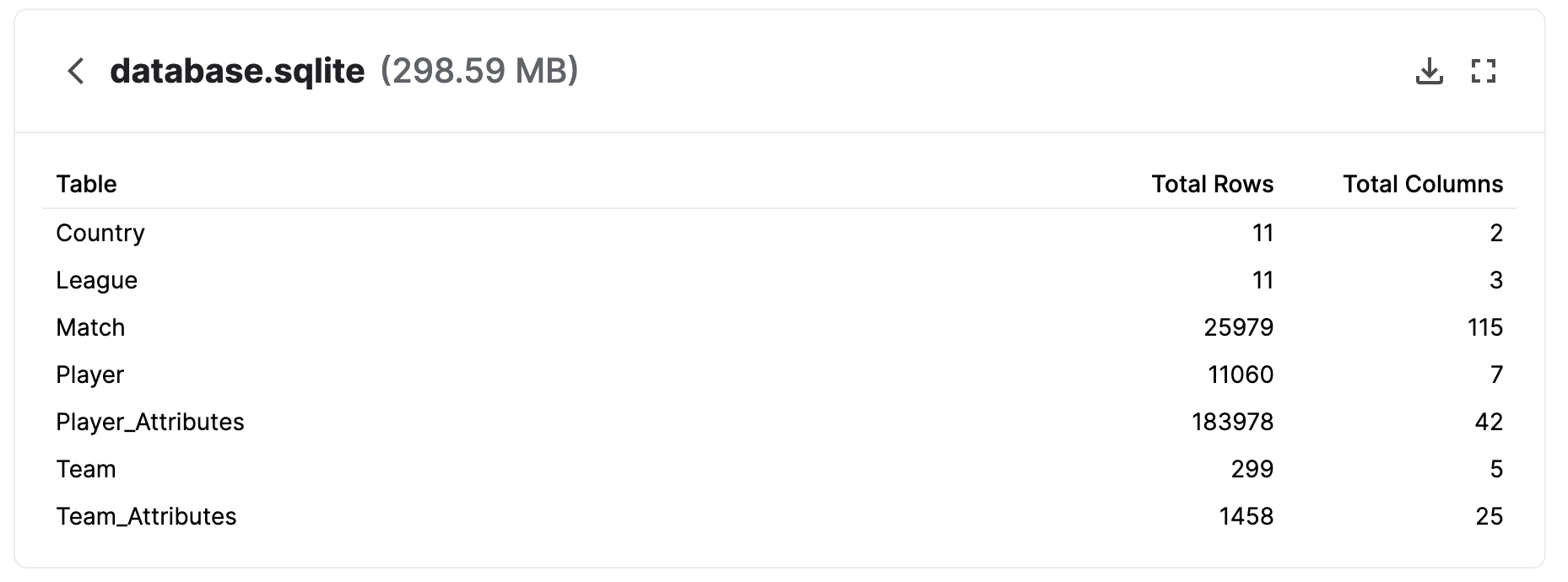
We use the League table to select Matches from the Spanish La Liga. Each match records the starting players for both home and away teams, so we merge these with Player Attributes to get the FIFA overall & potential ratings.
The resulting table looks like this (check the script for the whole data-processing pipeline):
| id | country_id | league_id | season | stage | date | home_team_goal | away_team_goal | match_api_id | home_team_api_id | away_team_api_id | home_player_1 | home_player_2 | home_player_3 | home_player_4 | home_player_5 | home_player_6 | home_player_7 | home_player_8 | home_player_9 | home_player_10 | home_player_11 | away_player_1 | away_player_2 | away_player_3 | away_player_4 | away_player_5 | away_player_6 | away_player_7 | away_player_8 | away_player_9 | away_player_10 | away_player_11 | B365H | B365D | B365A | BWH | BWD | BWA | IWH | IWD | IWA | LBH | LBD | LBA | PSH | PSD | PSA | WHH | WHD | WHA | SJH | SJD | SJA | VCH | VCD | VCA | GBH | GBD | GBA | BSH | BSD | BSA | home_result | target |
|---|---|---|---|---|---|---|---|---|---|---|---|---|---|---|---|---|---|---|---|---|---|---|---|---|---|---|---|---|---|---|---|---|---|---|---|---|---|---|---|---|---|---|---|---|---|---|---|---|---|---|---|---|---|---|---|---|---|---|---|---|---|---|---|---|
| 22278 | 21518 | 21518 | 2010/2011 | 1 | 2010-08-30 00:00:00 | 4 | 0 | 875448 | 9906 | 9869 | 182917 | 30689 | 56678 | 32656 | 33636 | 38821 | 37411 | 25924 | 33871 | 38460 | 37412 | 75195 | 150480 | 107929 | 101070 | 74752 | 38746 | 30273 | 38004 | 38886 | 24383 | 41294 | 1.53 | 4 | 6 | 1.53 | 3.8 | 6 | 1.5 | 3.8 | 5.7 | 1.5 | 3.5 | 6 | nan | nan | nan | 1.5 | 3.8 | 6 | 1.57 | 3.75 | 6 | 1.53 | 3.8 | 6 | 1.5 | 4 | 6 | 1.57 | 3.75 | 5.5 | 1 | win |
| 22279 | 21518 | 21518 | 2010/2011 | 1 | 2010-08-28 00:00:00 | 0 | 1 | 875451 | 10278 | 8315 | 37511 | 37470 | 33715 | 33609 | 24630 | 18376 | 24385 | nan | 96852 | 74772 | 37497 | 33764 | 33025 | 182224 | 37604 | 191136 | 37410 | 33024 | 96619 | 37408 | 33030 | 150832 | 2.5 | 3.25 | 2.8 | 2.55 | 3.2 | 2.65 | 2.6 | 3.1 | 2.5 | 2.5 | 3.2 | 2.5 | nan | nan | nan | 2.5 | 3.2 | 2.6 | 2.6 | 3.2 | 2.75 | 2.5 | 3.12 | 2.75 | 2.6 | 3.25 | 2.6 | 2.5 | 3.25 | 2.6 | -1 | loss |
| 22280 | 21518 | 21518 | 2010/2011 | 1 | 2010-08-29 00:00:00 | 0 | 3 | 875458 | 8696 | 8634 | 37579 | 75606 | 128037 | 37879 | 74435 | 26535 | 37512 | 46836 | 97319 | 38382 | 35638 | 32657 | 33988 | 37482 | 30738 | 34304 | 39854 | 154257 | 26146 | 30981 | 30909 | 30955 | 15 | 6 | 1.2 | 12.5 | 6 | 1.2 | 9 | 5 | 1.27 | 10 | 5 | 1.22 | nan | nan | nan | 11 | 5.5 | 1.22 | 13 | 6.5 | 1.2 | 15 | 6.5 | 1.2 | 13 | 6 | 1.2 | 11 | 5.5 | 1.22 | -1 | loss |
| 22281 | 21518 | 21518 | 2010/2011 | 1 | 2010-08-28 00:00:00 | 1 | 3 | 875459 | 9864 | 10267 | 33826 | 33843 | 188517 | 41707 | 163236 | 11758 | 24612 | 128870 | 23779 | 56819 | 51545 | 24494 | 34007 | 30276 | 30914 | 26403 | 108568 | 30666 | 37824 | 41468 | 32762 | 33028 | 2.88 | 3.3 | 2.4 | 2.85 | 3.3 | 2.35 | 2.7 | 3.2 | 2.4 | 2.8 | 3.2 | 2.2 | nan | nan | nan | 2.9 | 3.25 | 2.25 | 2.8 | 3.25 | 2.5 | 2.88 | 3.2 | 2.4 | 2.85 | 3.25 | 2.4 | 2.9 | 3.25 | 2.3 | -1 | loss |
| 22282 | 21518 | 21518 | 2010/2011 | 1 | 2010-08-29 00:00:00 | 0 | 0 | 875462 | 9783 | 8394 | 96651 | 33756 | 37451 | 70891 | 18853 | 37449 | 37793 | 114680 | 45744 | 31045 | 166111 | 30664 | 37754 | 33582 | 27668 | 150968 | 33635 | 30534 | 38403 | 164676 | 45457 | 8780 | 2.1 | 3.3 | 3.5 | 2.05 | 3.25 | 3.5 | 2 | 3.2 | 3.4 | 2 | 3.2 | 3.2 | nan | nan | nan | 1.91 | 3.3 | 3.75 | 2.1 | 3.2 | 3.6 | 2.05 | 3.25 | 3.5 | 2 | 3.3 | 3.6 | 2.05 | 3.25 | 3.4 | 0 | draw |
You may notice several float-valued features to the right of away_player_11 with abbreviated feature names. These are
betting odds that have been scraped from the web for each match. The database contains the home win/draw/loss odds
from several sports betting sites. For example, B365H -> Bet365 home win odds. The full list can be found
here.
We will create two additional time-series-based features, just for fun. The first is a binary flag that indicates whether the home team won the same fixture against the away team in the previous season. The second one measures the number of wins by the home team in the last five games (this includes games where the home team was on the away side).
def get_prev_year_result(row):
    """
    Binary flag of whether the home team won the same fixture the previous year
    """
    home_team_id = row['home_team_api_id']
    away_team_api_id = row['away_team_api_id']
    season = row['season']
    prev_season = '/'.join(map(lambda x: str(int(x) - 1), season.split('/')))
    df_prev = df_match_spain[
        (df_match_spain['home_team_api_id'] == home_team_id) &
        (df_match_spain['away_team_api_id'] == away_team_api_id) &
        (df_match_spain['season'] == prev_season)
    ]

    if df_prev.empty:
        return 0
    else:
        return 1 if df_prev['target'].values[0] == 'win' else 0

def get_recent_form(row):
    """
    Number of wins by the home team in the past 5 games
    """
    home_team_id = row['home_team_api_id']
    season = row['season']
    stage = row['stage']
    df_prev_matches = df_match_spain[
        (df_match_spain['season'] == season) &
        ((df_match_spain['home_team_api_id'] == home_team_id) |
         (df_match_spain['away_team_api_id'] == home_team_id)) &
        (df_match_spain['stage'].between(max(0, stage-5), max(0,stage-1)))
    ]

    if df_prev_matches.empty:
        return 0
    else:
        return sum(df_prev_matches['home_result'] == 'win')

# Create the time-series-based features
df_match_spain['prev_year_result'] = df_match_spain.apply(get_prev_year_result, axis=1)
df_match_spain['wins_past_five_games'] = df_match_spain.apply(get_recent_form, axis=1)
Finally, the target variable, home_result, is simply calculated by comparing
home_team_goal and away_team_goal.
df_match_spain['home_result'] = (df_match_spain['home_team_goal'] - df_match_spain['away_team_goal'])
df_match_spain['home_result'] = df_match_spain['home_result'].apply(lambda x: x/abs(x) if x != 0 else 0)
df_match_spain['target'] = df_match_spain['home_result'].map({0: 'draw', -1: 'loss', 1: 'win'})
The proportions of target tells us that home teams win 48% of the time, which aligns with
the win-rate of home teams in the whole dataset as mentioned by the author of the dataset.
Thus 48% will be the baseline accuracy to which we compare our Bayesian model performance.
print(df_match_spain['target'].value_counts(normalize=True))

win     0.4841
loss    0.2834
draw    0.2323
Name: target, dtype: float64
Modelling
For this blog post, the task is to predict $y$, or whether the home team won, drew, or lost a given match, and its variables, $x$.
We model these outcomes via logistic regression:
\[\begin{align*} E(y=1 |x, \beta) = & \qquad \textit{logit}^{-1}(u)\\ u = & \qquad \beta_{0} + \beta_{1}x_{1} \cdots + \beta_{k} x_{k}\\ \textit{logit}^{-1}(u) = & \qquad \frac{1}{1 + exp(-u)}\\ \end{align*}\]where $\beta$ are the parameters of the logistic regression, $x$ are the features of the match (betting odds, player attributes, etc.), and $\textit{logit}^{-1}$ is the sigmoid function.
When we have multiple outcomes, we simply divide the logits of each outcome (win, draw, loss), with the sum of all logits (i.e. softmax):
\[\begin{align*} \textit{CategoricalLogit}(y|\alpha) = & \qquad \textit{Categorical}(y|\textit{softmax}(\alpha))\\ \textit{softmax}(\alpha) = & \qquad \frac{exp(u)}{\sum^n exp(u)}\\ \end{align*}\]You may be wondering how this is any different from using the logistic regression model from Scikit-Learn. The logistic regression we’re familiar with learns its parameters $\beta$ by calculating the cross-entropy loss between its predictions and the groundtruth and then performing gradient descent to adjust its parameters.
Instead, today we will be taking a Bayesian approach to estimating optimal values of $\beta$.
Recall Bayes’ formula:
\[p(\beta | y) = \frac{p(y|\beta)p(\beta)}{p(y)}\]Does putting Bayes’ formula on my humble blog make me a Bayesian?
We want to estimate $\beta$, the parameters of our logistic regression model, using our observations of match outcomes $y$ (also called the posterior). The formula relates the posterior $p(y|\beta)$, the distribution of match outcomes given some estimate $\beta$, to $p(\beta)$, our prior beliefs on how $\beta$ is distributed, and $p(y)$, the distribution of match outcomes (aka the evidence).
While we can readily compute $p(y|\beta)$ and $p(\beta)$, the denominator requires computing $p(y) = \int p(y, \beta)d\beta$, which means we must compute $p(y, \beta)$ over all possible values of $\beta$, which is intractable.
We instead approximate $p(\beta | y)$ using Markov Chain Monte Carlo, a family of methods for sampling from probability distributions and is the goto method for problems like these.
Put simply, Markov Chain Monte Carlo involves generating parameters $\beta_t$ in a stochastic fashion (hence Monte Carlo) and deciding via some stochastic procedure whether $\beta_t$ succeeds $\beta_{t-1}$ for the next iteration (hence Markov Chain). If you are new to MCMC, I highly encourage you to check out how some of the popular MCMC algorithms work (e.g. Metropolis Hastings, Hamiltonian Monte Carlo). Some resources:
Our implementation relies on PyStan, a Python wrapper around Stan, one of the most widely used open-source probabalistic programming frameworks. Apart from robust documenation and community support, Stan’s popularity can be attributed to an efficient and robust implementation of MCMC (known as NUTS, No U-Turn Sampler).
Stan code requires defining several blocks that define the data and model, compiling the model, and then fitting the parameters by running MCMC. These blocks usually include:
- Data: defining input data types and shapes
- Parameters: defining parameters of the model which will be learned
- Model: defining how we model the data, i.e. how the observed data (match outcomes) are related to the parameters
Here is our Stan definition of our simple logistic regression model:
stan_model = '''

data {
  int N; // the number of training observations
  int N2; // the number of test observations
  int D; // the number of features
  int K; // the number of classes
  int y[N]; // the response
  matrix[N,D] x; // training data
  matrix[N2,D] x_test; //the matrix for the predicted values
}

parameters {
  matrix[D,K] beta; // the regression parameters
}

model {
  matrix[N, K] x_beta = x * beta; // linear component of logistic regression
  to_vector(beta) ~ normal(0, 1); // our prior on beta

  for (n in 1:N)
    y[n] ~ categorical_logit(x_beta[n]'); // the inverse logit function

}

generated quantities {
    vector[N2] y_new;
    matrix[N2, K] x_beta_new = x_test * beta;
    for (n in 1:N2)
        y_new[n] = categorical_rng(softmax(x_beta_new[n]'));
}

'''
The model block represents our definition of our logistic regression model.
Note that we can set a prior for beta - we are essentially assuming that the
learned beta parameters will follow a normal distribution. We will verify this later!
The generated quantities block is where we generate predictions for our test data
with our trained parameters. You can find Stan documentation on logistic regression
here and
here.
We then compile the model:
sm = stan.StanModel(model_code=stan_model, model_name='la_liga_model')
Finally, we prepare our data and call fit:
target_col = "home_result"
df_features = df_match_spain[list_features]
df_features[target_col] = df_features['home_result'].map({-1: 1, 0: 2, 1:3})

X = df_features.drop(columns=target_col).values
y = df_features[target_col].values

print(X.shape) # (1898, 64)
print(y.shape) # (1898, )

# Split the data
X_train, X_test, y_train, y_test = train_test_split(X, y, test_size=0.2, random_state=SEED)

# MinMax scaling
sc = MinMaxScaler()
X_train = sc.fit_transform(X_train)
X_test = sc.transform(X_test)

#The sampling methods in PyStan require the data to be input as a Python dictionary whose keys match
#the data block of the Stan code.
data = dict(
    N = X_train.shape[0],
    N2 = X_test.shape[0],
    D = X_train.shape[1],
    K = len(set(y_train)),
    y = y_train,
    x = X_train,
    x_test = X_test,
)

# Fit
fit = sm.sampling(data=data, chains=5, iter=2000, warmup=1000, control=dict(max_treedepth=15))
How do we know whether our model has converged? We can inspect results by simply
running print(fit):
Inference for Stan model: LaLiga_time_series_632fd94a6fffdb66823909d28b95e85f.
5 chains, each with iter=2000; warmup=1000; thin=1;
post-warmup draws per chain=1000, total post-warmup draws=5000.

              mean se_mean     sd   2.5%     25%     50%    75%  97.5%  n_eff   Rhat
beta[1,1]     0.38  9.1e-3   0.93   -1.4   -0.25    0.39   1.04   2.14  10374    1.0
beta[2,1]   1.6e-3  8.9e-3   0.98  -1.98   -0.65 -9.2e-3   0.65   1.99  12155    1.0
beta[3,1]    -0.14  9.8e-3   0.97  -2.05   -0.81   -0.15   0.52   1.77   9937    1.0
beta[4,1]      0.3  9.0e-3   0.97  -1.58   -0.36    0.31   0.97   2.22  11773    1.0
beta[5,1]     0.02  9.6e-3   0.97  -1.95   -0.63    0.02   0.68    1.9  10294    1.0
beta[6,1]    -0.29  8.6e-3   0.95  -2.19   -0.92   -0.28   0.35   1.58  12159    1.0
beta[7,1]     0.07  8.2e-3   0.93  -1.77   -0.57    0.07   0.72    1.9  12851    1.0
beta[8,1]    -0.13  8.8e-3   0.93  -1.94   -0.75   -0.13    0.5   1.72  11132    1.0
beta[9,1]    -0.04  8.9e-3   0.91  -1.78   -0.67   -0.05   0.57   1.74  10489    1.0
beta[10,1]    0.48  9.2e-3   0.94  -1.32   -0.17    0.46    1.1   2.35  10547    1.0
beta[11,1]    0.01  9.0e-3   0.95  -1.87   -0.62  3.6e-3   0.65   1.88  11238    1.0
beta[12,1]   -0.28  9.8e-3   0.96  -2.18   -0.92   -0.28   0.38   1.58   9593    1.0
beta[13,1]    0.25  9.0e-3   0.95  -1.62   -0.38    0.26   0.89   2.12  11137    1.0
beta[14,1]    -0.1  9.8e-3   0.95  -1.93   -0.76   -0.11   0.56    1.8   9498    1.0
beta[15,1]   -0.33  9.0e-3    1.0  -2.31   -0.99   -0.34   0.33   1.63  12113    1.0
beta[16,1]    0.31  9.2e-3   0.95  -1.56    -0.3     0.3   0.94   2.21  10671    1.0
beta[17,1]    0.07  8.6e-3   0.97  -1.81   -0.61    0.07   0.74   1.97  12634    1.0
beta[18,1]   -0.11  9.7e-3   0.95  -1.99   -0.76   -0.12   0.52   1.75   9671    1.0
beta[19,1]    0.37  8.8e-3   0.72  -1.05   -0.12    0.36   0.85   1.79   6614    1.0
beta[20,1]   -0.67  9.3e-3   0.71  -2.02   -1.15   -0.66  -0.19   0.71   5767    1.0
beta[21,1]   -0.43  9.1e-3   0.71  -1.83   -0.91   -0.43   0.05   0.99   6150    1.0
beta[22,1]   -0.46  9.0e-3   0.72  -1.88   -0.94   -0.46   0.02   0.97   6452    1.0
beta[23,1]   -0.28  9.1e-3   0.72  -1.71   -0.76   -0.26    0.2   1.16   6235    1.0
beta[24,1]    0.38  9.9e-3   0.64  -0.87   -0.05    0.39   0.82   1.66   4214    1.0
beta[25,1]    0.16  8.6e-3    0.7  -1.23   -0.31    0.15   0.64   1.53   6554    1.0
beta[26,1]   -0.68  9.8e-3   0.68  -1.97   -1.13    -0.7  -0.23   0.66   4828    1.0
beta[27,1]   -0.08  8.1e-3   0.75  -1.57   -0.58   -0.07   0.41    1.4   8563    1.0
beta[28,1]    0.35  9.4e-3   0.67  -0.97    -0.1    0.34    0.8   1.63   5124    1.0
beta[29,1]    0.23  8.5e-3   0.75  -1.27   -0.27    0.22   0.73   1.73   7729    1.0
beta[30,1]   -0.41  8.8e-3    0.7  -1.78   -0.88   -0.39   0.07   0.96   6234    1.0
beta[31,1]   -0.47  8.9e-3   0.74  -1.89   -0.97   -0.48   0.02   0.94   6876    1.0
beta[32,1]    0.42  9.1e-3   0.69  -0.93   -0.05     0.4   0.87   1.76   5661    1.0
beta[33,1]    0.16  9.4e-3   0.71  -1.24   -0.32    0.16   0.65   1.56   5741    1.0
beta[34,1]   -0.07  9.0e-3   0.68   -1.4   -0.53   -0.07    0.4   1.24   5821    1.0
beta[35,1]   -0.66  8.3e-3   0.74  -2.09   -1.16   -0.65  -0.16   0.81   7921    1.0
beta[36,1] -1.7e-3  8.8e-3   0.71  -1.35   -0.47   -0.01   0.47   1.43   6476    1.0
beta[37,1]   -0.07  9.2e-3   0.71  -1.46   -0.56   -0.07   0.41   1.34   5990    1.0
beta[38,1]    0.13  8.8e-3    0.7   -1.2   -0.34    0.11   0.61   1.52   6299    1.0
beta[39,1]   -0.18  8.9e-3   0.73  -1.58   -0.68    -0.2    0.3   1.25   6689    1.0
beta[40,1]   -0.33  9.3e-3   0.71   -1.7   -0.82   -0.33   0.16   1.09   5846    1.0
beta[41,1]    0.17  9.3e-3   0.72  -1.25   -0.32    0.17   0.66   1.58   6077    1.0
beta[42,1]   -0.13  9.4e-3   0.68   -1.5   -0.58   -0.12   0.33   1.19   5327    1.0
beta[43,1]    0.37  9.3e-3   0.73  -1.05   -0.11    0.37   0.85   1.77   6103    1.0
beta[44,1]    0.38  9.3e-3   0.72  -1.03   -0.11    0.38   0.87   1.78   6016    1.0
beta[45,1]    0.14  8.8e-3   0.71  -1.23   -0.32    0.15   0.61   1.51   6384    1.0
beta[46,1]    0.01  9.5e-3   0.69  -1.36   -0.46    0.02   0.48   1.35   5277    1.0
beta[47,1]   -0.11  8.9e-3   0.74  -1.59   -0.59   -0.12   0.38   1.35   6795    1.0
beta[48,1]    0.45  9.0e-3   0.67  -0.85 -1.9e-3    0.46    0.9   1.74   5461    1.0
beta[49,1]    0.43  8.4e-3   0.71  -0.97   -0.06    0.45   0.92   1.78   7231    1.0
beta[50,1]    0.53  9.4e-3   0.68  -0.78    0.06    0.53   0.99   1.87   5329    1.0
beta[51,1]    0.02  8.8e-3   0.76  -1.46    -0.5    0.02   0.54   1.47   7333    1.0
beta[52,1]    0.51  8.7e-3   0.72  -0.89    0.03     0.5    1.0   1.93   6900    1.0
beta[53,1]   -0.08  9.5e-3   0.74  -1.54   -0.59   -0.08   0.42   1.37   6201    1.0
beta[54,1]   -0.59  9.3e-3    0.7  -1.97   -1.06   -0.59  -0.12   0.79   5650    1.0
beta[55,1]    0.11  9.0e-3   0.74  -1.31   -0.39     0.1    0.6   1.56   6864    1.0
beta[56,1]    0.06  9.6e-3   0.73  -1.36   -0.43    0.05   0.54   1.49   5715    1.0
beta[57,1]    0.42  8.5e-3   0.75  -1.04   -0.08    0.41   0.92   1.92   7820    1.0
beta[58,1]    0.08  9.1e-3   0.72  -1.37   -0.41    0.08   0.57   1.44   6310    1.0
beta[59,1]    0.06  9.0e-3   0.72  -1.34   -0.43    0.07   0.55   1.45   6420    1.0
beta[60,1]   -0.04  8.8e-3   0.71  -1.43   -0.51   -0.04   0.43   1.32   6506    1.0
beta[61,1]   -0.31  8.5e-3   0.71  -1.71    -0.8    -0.3   0.17   1.06   7027    1.0
beta[62,1]    -0.1  9.2e-3   0.71  -1.47   -0.57    -0.1   0.38   1.29   5839    1.0
beta[63,1]    -0.1  9.9e-3    0.6  -1.29   -0.49    -0.1   0.31   1.07   3724    1.0
beta[64,1]    -0.1    0.01   0.59  -1.28    -0.5   -0.09    0.3   1.02   3476    1.0
...
beta[59,3]    -0.3  9.0e-3    0.7  -1.65   -0.78   -0.31   0.19   1.06   6193    1.0
beta[60,3]    0.19  8.7e-3   0.69  -1.16   -0.27    0.18   0.67   1.56   6357    1.0
beta[61,3]    0.11  9.1e-3   0.72  -1.28   -0.39     0.1   0.58   1.52   6257    1.0
beta[62,3]   -0.05  9.3e-3   0.69  -1.33   -0.52   -0.04   0.41   1.31   5522    1.0
beta[63,3]    0.05    0.01    0.6  -1.12   -0.37    0.04   0.46   1.21   3600    1.0
beta[64,3]    0.04    0.01   0.59  -1.15   -0.35    0.06   0.44   1.16   3482    1.0
lp__         -1463    0.22   9.78  -1482   -1469   -1462  -1456  -1444   1976    1.0

Samples were drawn using NUTS at Sat May  15 16:51:02 2021.
For each parameter, n_eff is a crude measure of effective sample size,
and Rhat is the potential scale reduction factor on split chains (at
convergence, Rhat=1).
Each row represents a value of our parameter beta (except lp__, which is a meta parameter for log densities).
The columns display statistics about each parameter. The last column, Rhat, or also known
as the Potential Scale Reduction Factor (Vehtari et al., 2021), indicates whether or
not MCMC failed to converge. It measures the ratio between between-chains and within-chains estimates of parameters,
hence having a ratio closer to 1.0 means that the chains have “mixed” relatively well.
Here’s a visualization of our model parameters using the ArviZ package, a visualization utility for Bayesian data analysis.
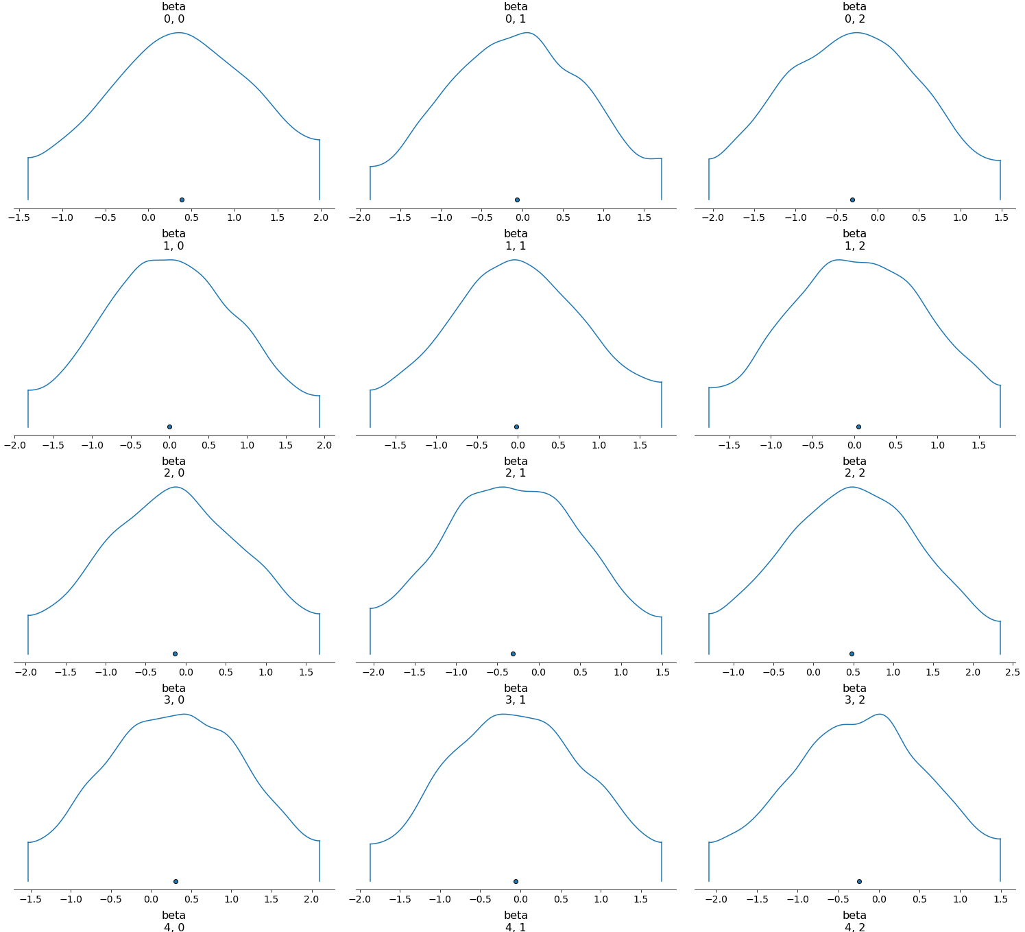
As the figure shows, our beta indeed follow a normal distribution, confirming that we have
selected an appropriate prior distribution of beta.
Evaluation and Visualizations
Now that we have our fitted PyStan model, we can measure its performance on test data and compare it with other approaches.
Accuracy vs. baseline and LightGBM
Let’s first extract the predictions from the model.
samples = fit.extract()
y_pred = samples['y_new']

print(y_pred.shape) # (5000, 380)

y_pred = scipy.stats.mode(y_pred, axis=0).mode.ravel()
For each test instance (380 in total), we sample 5,000 estimates from MCMC. We aggregate the estimates by taking the mode, or seeing which outcome (1: loss, 2: draw, 3: win) had the most “votes”.
Here’s the classification report:
                  precision    recall  f1-score   support

           1       0.50      0.54      0.52        98
           2       0.18      0.03      0.05        93
           3       0.60      0.81      0.69       189

accuracy                               0.55       380
macro avg          0.43      0.46      0.42       380
weighted avg       0.47      0.55      0.49       380
Recall that the baseline was 48%, or the proportion of wins among all labels. Our accuracy of 55% suggests that our model performance exceeds this.
We also measure the performance of a LightGBM model on the same dataset:
                    precision    recall  f1-score   support

            1       0.52      0.48      0.50        98
            2       0.31      0.12      0.17        93
            3       0.60      0.80      0.69       189

accuracy                                0.55       380
macro avg           0.47      0.47      0.45       380
weighted avg        0.51      0.55      0.51       380
LightGBM seems to predict draws better, but apart from that our Bayesian logistic regressions seems to perform as well as LightGBM! This was somewhat unexpected - perhaps this is because we are using a limited set of features.
What if we select the most confident predictions?
Bayesian data analysis is useful because we get uncertainty estimates of the statistics we care about. In other words, our model can tell us whether it’s confident about a particular prediction or not.
What if we choose the most confident predictions (i.e. the chances of the home team winning are really high)? To simplify this investigation, we convert our multi-class logistic regression to a binary one (both draw and loss grouped into one label). PyStan-wise, this requires minor changes to the model:
stan_model = '''

data {
    int<lower=0> N;
    int<lower=0> K;
    matrix[N, K] Q;
    int y[N];
}

parameters {
    real alpha; // intercept
    vector [K] theta; // coefficients
}

model {
    y ~ bernoulli_logit(Q * theta + alpha);  // posterior
}

'''
The classification report for the entire test set (380 samples) look like this:
                precision    recall  f1-score   support

            0       0.64      0.78      0.70       191
            1       0.72      0.56      0.63       189

accuracy                                0.67       380
macro avg           0.68      0.67      0.67       380
weighted avg        0.68      0.67      0.67       380
Here is how accuracy changes when we get the accuracy for each 10%-tile range of predictions based on confidence:
| Confidence percentile (%-ile) | Accuracy (%) |
|---|---|
| 90~100 | 89.47 |
| 80~90 | 73.15 |
| 70~80 | 68.42 |
| 60~70 | 68.42 |
| 50~60 | 47.36 |
| 40~50 | 52.63 |
| 30~40 | 60.52 |
| 20~30 | 71.05 |
| 10~20 | 68.42 |
| 0~10 | 81.57 |
Accuracy seems to vary drastically depending on how confident the model is. At the extremes (90~100% -> model confident that the home team will win; 0~10% -> model confident that the home team will not), we exceed 80% accuracy, but in the realm of ambivalence (confidence percentile 40~60%), that drops down to 47%.
This tells us that to some extent the model’s confidence can be intepreted as how reliable the prediction is. This is important in practice/industry; if we were to actually place bets on particular outcomes, we would prefer predictions where the model is very confident.
Visualizations
We will wrap this blog post up with some visualizations.
First off, let’s compare the posteriors of the stronger teams in La Liga (FC Barcelona, Real Madrid, and Atletico Madrid) to mid/low-table clubs.
def calculate_posteriors(X_features, theta, alpha):
    outcomes = np.dot(theta, np.transpose(X_features))
    print(outcomes.shape)

    for j in range(outcomes.shape[1]):
        outcomes[:, j] = scipy.special.expit(outcomes[:, j] + alpha)

    outcomes = np.transpose(outcomes)
    return outcomes

team_colors = [
    "#004C99",
    "#FFFFFF",
    "#CB3524",
    "#FCED0B",
    "#007c66",
    "#c86c05",
]

list_teams = [
    "BAR",
    "REA",
    "AMA",
    "GET",
    "RAY",
    "ALM",
]

dict_team_to_id = df_team_spain.set_index("team_short_name")["team_api_id"].to_dict()
dict_team_to_long = df_team_spain.set_index("team_short_name")["team_long_name"].to_dict()
list_team_ids = [dict_team_to_id[t] for t in list_teams]

theta = samples["theta"]
alpha = samples["alpha"]

list_buf = []
for team in tqdm(list_teams):
    team_id = dict_team_to_id[team]

    df_matches_team = df_match_spain[df_match_spain["home_team_api_id"] == team_id].sample(10)
    df_features_team = df_matches_team[list_features]
    df_features_team = df_features_team.drop(columns=target_col)
    X_features = sc.transform(df_features_team.values)
    outcomes = calculate_posteriors(X_features, theta, alpha)

    df_post = pd.DataFrame({"posteriors": outcomes.ravel()})
    df_post["team"] = dict_team_to_long[team]
    list_buf.append(df_post)

df_posteriors = pd.concat(list_buf)

sns.set_theme(style="whitegrid")
plt.figure(figsize=(15,8))
sns.set_context('paper', font_scale=2.5)
sns.set_palette(team_colors)

ax = sns.violinplot(y="team", x="posteriors", data=df_posteriors, scale="width", orient="h")
ax.set(ylabel="", xlabel="Posterior", title="Home team win probability distribution")
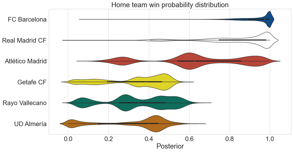
The model recognizes that the three strongest teams in the league often have a higher chance of winning compared to its peers.
What do the posteriors look like when we pit one club (FC Barcelona) against its peers?
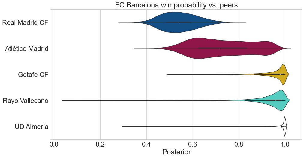
As one may expect, FC Barcelona vs. Real Madrid is usually a toss-up. It is favored over Atletico Madrid in most matches and is almost guaranteed a victory by the model against the bottom half of the league.
Finally, here’s a visualization of how betting odds affect the posterior.
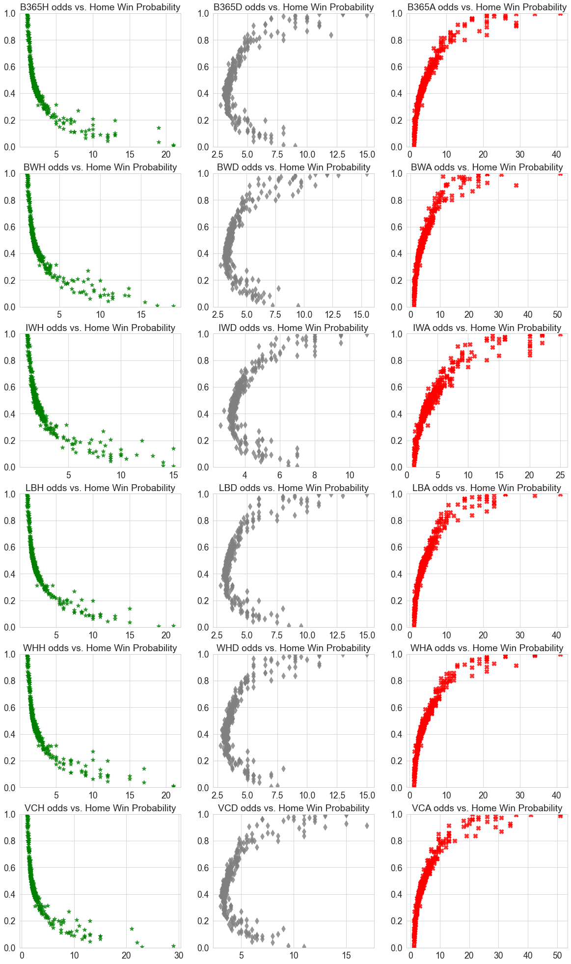
It follows our intuition that the lower the winning odds (green) are, the higher the posterior, and vice versa for away winning odds (red). For drawing odds (grey), we see a C-shaped curve; if the odds of drawing are high, then the game would either end in a home win or loss.
Summary
Thanks for making it this far! In this blog post, we used PyStan to implement a Bayesian logistic regression model and predict Spanish football matches based on betting odds & player attributes based on FIFA ratings. Not only does our simple model perform comparatively to a LightGBM model, we are able to extract insights related to individual teams and variables based from the posterior.
There’s a lot more that one can do with PyStan (e.g. hierarchical modelling), so I hope to implement a more complex model next time.
I will sign off by sharing some additional for those of you curious about how MCMC works.
- The Markov Chain Monte Carlo Revolution
- MCMC using Hamiltonian Dynamics
- A Conceptual Introduction to Hamiltonian Monte Carlo
PyStanでサッカーの試合結果を予測してみた
はじめに
現職に就いてから早9ヶ月が経ちました。当たり前のことかもしれませんが、インダストリーにおけるデータサイエンスでは accuracyなどのアカデミックな指標よりも、ビジネス・社会におけるインパクトをより重視していることが 顕著です。データ・結果を理解し既存のビジネスプロセス・判断の効率・精度を上げることが分析の目的の一つとも言えます。
従って、分析に使われる手法も人間による解釈がしやすいものが多かったりします。その一つとしてベイズなどを 使った確率的プログラミングが挙げられます。本記事では独学の一環としてPyStanというベイズモデリングのパッケージを 使って実データを分析してみたいと思います。
本記事の構成は以下の通りです。
- データの解説、前処理
- モデリング
- 評価、可視化
データ
今回の分析にはKaggle上にある European Soccer Database というデータセットを用います。データの概要をざっと説明すると、
- データの期間:2008~2016
- 11個の欧州サッカーリーグ及び25,000以上の試合情報
- 10,000以上の選手情報
- 10社のブックメーカーによる各試合のオッズ情報
- FIFA(ゲームの方)における各選手の特徴、レーティング
などが情報として入っている、かなりしっかりしたものです。今回は使用データを2010年以降のスペイン1部リーグ(ラ・リーガ)の 試合に限定し、特徴量として使う項目も1)ブックメーカーのオッズ、2)FIFAの選手レーティングに絞って分析を 回してみたいと思います。目的変数は、ホームチームの勝利、引き分け、敗北の三択です。
では先ずは簡単な前処理でデータを整えましょう。データセット内は以下のsqliteテーブルが入っています。
今回使うのはLeague、Match、Player Attributesのみなので、それらをラ・リーガに該当するものに絞りながら マージします。マージ後はこんな感じです。
| id | country_id | league_id | season | stage | date | home_team_goal | away_team_goal | match_api_id | home_team_api_id | away_team_api_id | home_player_1 | home_player_2 | home_player_3 | home_player_4 | home_player_5 | home_player_6 | home_player_7 | home_player_8 | home_player_9 | home_player_10 | home_player_11 | away_player_1 | away_player_2 | away_player_3 | away_player_4 | away_player_5 | away_player_6 | away_player_7 | away_player_8 | away_player_9 | away_player_10 | away_player_11 | B365H | B365D | B365A | BWH | BWD | BWA | IWH | IWD | IWA | LBH | LBD | LBA | PSH | PSD | PSA | WHH | WHD | WHA | SJH | SJD | SJA | VCH | VCD | VCA | GBH | GBD | GBA | BSH | BSD | BSA | home_result | target |
|---|---|---|---|---|---|---|---|---|---|---|---|---|---|---|---|---|---|---|---|---|---|---|---|---|---|---|---|---|---|---|---|---|---|---|---|---|---|---|---|---|---|---|---|---|---|---|---|---|---|---|---|---|---|---|---|---|---|---|---|---|---|---|---|---|
| 22278 | 21518 | 21518 | 2010/2011 | 1 | 2010-08-30 00:00:00 | 4 | 0 | 875448 | 9906 | 9869 | 182917 | 30689 | 56678 | 32656 | 33636 | 38821 | 37411 | 25924 | 33871 | 38460 | 37412 | 75195 | 150480 | 107929 | 101070 | 74752 | 38746 | 30273 | 38004 | 38886 | 24383 | 41294 | 1.53 | 4 | 6 | 1.53 | 3.8 | 6 | 1.5 | 3.8 | 5.7 | 1.5 | 3.5 | 6 | nan | nan | nan | 1.5 | 3.8 | 6 | 1.57 | 3.75 | 6 | 1.53 | 3.8 | 6 | 1.5 | 4 | 6 | 1.57 | 3.75 | 5.5 | 1 | win |
| 22279 | 21518 | 21518 | 2010/2011 | 1 | 2010-08-28 00:00:00 | 0 | 1 | 875451 | 10278 | 8315 | 37511 | 37470 | 33715 | 33609 | 24630 | 18376 | 24385 | nan | 96852 | 74772 | 37497 | 33764 | 33025 | 182224 | 37604 | 191136 | 37410 | 33024 | 96619 | 37408 | 33030 | 150832 | 2.5 | 3.25 | 2.8 | 2.55 | 3.2 | 2.65 | 2.6 | 3.1 | 2.5 | 2.5 | 3.2 | 2.5 | nan | nan | nan | 2.5 | 3.2 | 2.6 | 2.6 | 3.2 | 2.75 | 2.5 | 3.12 | 2.75 | 2.6 | 3.25 | 2.6 | 2.5 | 3.25 | 2.6 | -1 | loss |
| 22280 | 21518 | 21518 | 2010/2011 | 1 | 2010-08-29 00:00:00 | 0 | 3 | 875458 | 8696 | 8634 | 37579 | 75606 | 128037 | 37879 | 74435 | 26535 | 37512 | 46836 | 97319 | 38382 | 35638 | 32657 | 33988 | 37482 | 30738 | 34304 | 39854 | 154257 | 26146 | 30981 | 30909 | 30955 | 15 | 6 | 1.2 | 12.5 | 6 | 1.2 | 9 | 5 | 1.27 | 10 | 5 | 1.22 | nan | nan | nan | 11 | 5.5 | 1.22 | 13 | 6.5 | 1.2 | 15 | 6.5 | 1.2 | 13 | 6 | 1.2 | 11 | 5.5 | 1.22 | -1 | loss |
| 22281 | 21518 | 21518 | 2010/2011 | 1 | 2010-08-28 00:00:00 | 1 | 3 | 875459 | 9864 | 10267 | 33826 | 33843 | 188517 | 41707 | 163236 | 11758 | 24612 | 128870 | 23779 | 56819 | 51545 | 24494 | 34007 | 30276 | 30914 | 26403 | 108568 | 30666 | 37824 | 41468 | 32762 | 33028 | 2.88 | 3.3 | 2.4 | 2.85 | 3.3 | 2.35 | 2.7 | 3.2 | 2.4 | 2.8 | 3.2 | 2.2 | nan | nan | nan | 2.9 | 3.25 | 2.25 | 2.8 | 3.25 | 2.5 | 2.88 | 3.2 | 2.4 | 2.85 | 3.25 | 2.4 | 2.9 | 3.25 | 2.3 | -1 | loss |
| 22282 | 21518 | 21518 | 2010/2011 | 1 | 2010-08-29 00:00:00 | 0 | 0 | 875462 | 9783 | 8394 | 96651 | 33756 | 37451 | 70891 | 18853 | 37449 | 37793 | 114680 | 45744 | 31045 | 166111 | 30664 | 37754 | 33582 | 27668 | 150968 | 33635 | 30534 | 38403 | 164676 | 45457 | 8780 | 2.1 | 3.3 | 3.5 | 2.05 | 3.25 | 3.5 | 2 | 3.2 | 3.4 | 2 | 3.2 | 3.2 | nan | nan | nan | 1.91 | 3.3 | 3.75 | 2.1 | 3.2 | 3.6 | 2.05 | 3.25 | 3.5 | 2 | 3.3 | 3.6 | 2.05 | 3.25 | 3.4 | 0 | draw |
away_player_11という列以降の略語みたいな項目がオッズ情報になります。例えばB365Hだと
「Bet365社によるホームチーム勝利のオッズ」が入っています。各オッズ項目の対応表は
こちらをご参照ください。
これだけデータが揃っているので折角なので時系列情報も入れたいと思います(追加する列は2つだけですが)。 一つ目は、前年同カードでホームチームが勝ったかどうか。二つ目は、直近5試合におけるホームチームの勝利数 (ホームチームがアウェイだった試合も含む)を計算します。
def get_prev_year_result(row):
    """
    Binary flag of whether the home team won the same fixture the previous year
    """
    home_team_id = row['home_team_api_id']
    away_team_api_id = row['away_team_api_id']
    season = row['season']
    prev_season = '/'.join(map(lambda x: str(int(x) - 1), season.split('/')))
    df_prev = df_match_spain[
        (df_match_spain['home_team_api_id'] == home_team_id) &
        (df_match_spain['away_team_api_id'] == away_team_api_id) &
        (df_match_spain['season'] == prev_season)
    ]

    if df_prev.empty:
        return 0
    else:
        return 1 if df_prev['target'].values[0] == 'win' else 0

def get_recent_form(row):
    """
    Number of wins by the home team in the past 5 games
    """
    home_team_id = row['home_team_api_id']
    season = row['season']
    stage = row['stage']
    df_prev_matches = df_match_spain[
        (df_match_spain['season'] == season) &
        ((df_match_spain['home_team_api_id'] == home_team_id) |
         (df_match_spain['away_team_api_id'] == home_team_id)) &
        (df_match_spain['stage'].between(max(0, stage-5), max(0,stage-1)))
    ]

    if df_prev_matches.empty:
        return 0
    else:
        return sum(df_prev_matches['home_result'] == 'win')

# Create the time-series-based features
df_match_spain['prev_year_result'] = df_match_spain.apply(get_prev_year_result, axis=1)
df_match_spain['wins_past_five_games'] = df_match_spain.apply(get_recent_form, axis=1)
最後に、目的変数を計算します。
df_match_spain['home_result'] = (df_match_spain['home_team_goal'] - df_match_spain['away_team_goal'])
df_match_spain['home_result'] = df_match_spain['home_result'].apply(lambda x: x/abs(x) if x != 0 else 0)
df_match_spain['target'] = df_match_spain['home_result'].map({0: 'draw', -1: 'loss', 1: 'win'})
targetの分布を見ると、ホームチームが48%の確率で勝利していることが分かります。こちらは後ほど
モデル評価のベースラインとして使う予定です。
print(df_match_spain['target'].value_counts(normalize=True))

win     0.4841
loss    0.2834
draw    0.2323
Name: target, dtype: float64
モデリング
さて、データが整ったところでモデリングに移りたいと思います。今回はベイジアン・ロジスティック回帰という モデルを学習します。目的変数(勝ったか、負けたか、引き分けたか)を$y$、特徴量を$x$とすると、 数式的には以下のように表せます。
\[\begin{align*} E(y=1 |x, \beta) = & \qquad \textit{logit}^{-1}(u)\\ u = & \qquad \beta_{0} + \beta_{1}x_{1} \cdots + \beta_{k} x_{k}\\ \textit{logit}^{-1}(u) = & \qquad \frac{1}{1 + exp(-u)}\\ \end{align*}\]$\beta$がロジスティック回帰のパラメータ、$\textit{logit}^{-1}$がシグモイド関数となっております。
多クラス分類器の場合は、softmax関数を使ってlogitsを正規化します。
\[\begin{align*} \textit{CategoricalLogit}(y|\alpha) = & \qquad \textit{Categorical}(y|\textit{softmax}(\alpha))\\ \textit{softmax}(\alpha) = & \qquad \frac{exp(u)}{\sum^n exp(u)}\\ \end{align*}\]ここまでだと「Scikit-learnにもあるロジスティック回帰とは何が違うんだろう」と思ってらっしゃる 方もいるかと思います。Scikit-learnにおけるロジスティック回帰のパラメータ$\beta$は基本的に 交差エントロピー・ロス関数を最小化することによって学習しております。
それに対して、今回使うベイジアン・ロジスティック回帰では別の手法を用いてパラメータを学習しています。 教科書通りですが、ベイズの定理を使ってロジスティック回帰のパラメータを表すと下記のようになります。
\[p(\beta | y) = \frac{p(y|\beta)p(\beta)}{p(y)}\]データ$y$に条件付けされた学習パラメータ$\beta$(事後分布)を、$p(y|\beta)$(尤度)及び $\beta$の分布$p(\beta)$(事前分布)などで求めるというお馴染みに構図ですが、ここでネックになるのが 分母・エビデンスとなる$p(y)$です。
尤度・事前分布は比較的容易にコンピュータで算出できるのに対して、エビデンスは $p(y) = \int p(y, \beta)d\beta$で表されるように、全ての$\beta$に対して$p(y, \beta)$を 算出する必要があり、基本的にはコンピュータの容量を超える処理量になってしまいます。言い換えれば、 学習したい確率分布($p(y|\beta)$)から直接乱数を生成するのは難しいのです。
そこで登場するのがマルコフ連鎖モンテカルロ法(MCMC)です。超シンプルにまとめると、求める確率分布に近似する サンプルを生成するアルゴリズムの総称であり、一歩深堀すると時間ステップ$t$ごとに ある確率的手順に従って$\beta_t$を算出し、これを重ねることによって 事後分布に従うような適切なマルコフ連鎖($\beta_{t-2}, \beta_{t-1}, \beta_t, \beta_{t+1}$を作成し、 マルコフ連鎖自体を幾つも生成することによって求める確率分布の標本となり得るサンプルを作る、といった手法です。 MCMCにもメトロポリス・ヘイスティングス法や、ハミルトニアン・モンテカルロ法など色々あります。ご参考までに MCMC関連の文献を記載します。
さて、MCMCの実装に関してですが、ようやくここで冒頭で述べたPyStanが登場してきます。 PyStanはStanという、業界・アカデミアで最も利用されている確率的プログラミングライブラリのPython wrapperです。 ドキュメンテーションがしっかりしていて、コミュニティが活発な他、No U-Turn Sampler(NUTS)という MCMCの高速かつrobustな実装を備えていることが人気の理由として挙げられます。
Stanでは基本的に以下の3つを予め定義し、モデルをコンパイルしてから学習します。
- データ:入力データの型及び形
- パラメータ:モデルの学習パラメータの定義(事前分布など)
- モデル:求める確率分布とパラメータの紐付き、モデルの定義など
今回使うベイジアン・ロジスティック回帰のStan定義は以下のようになります。
stan_model = '''

data {
  int N; // the number of training observations
  int N2; // the number of test observations
  int D; // the number of features
  int K; // the number of classes
  int y[N]; // the response
  matrix[N,D] x; // training data
  matrix[N2,D] x_test; //the matrix for the predicted values
}

parameters {
  matrix[D,K] beta; // the regression parameters
}

model {
  matrix[N, K] x_beta = x * beta; // linear component of logistic regression
  to_vector(beta) ~ normal(0, 1); // our prior on beta

  for (n in 1:N)
    y[n] ~ categorical_logit(x_beta[n]'); // the inverse logit function

}

generated quantities {
    vector[N2] y_new;
    matrix[N2, K] x_beta_new = x_test * beta;
    for (n in 1:N2)
        y_new[n] = categorical_rng(softmax(x_beta_new[n]'));
}

'''
modelブロックにあるbetaが前述の学習パラメータとなります。
to_vector(beta) ~ normal(0, 1)とう記述で、betaの事前分布が$N(0, 1)$の正規分布に
従うということを定義しています。
generated quantitiesでは学習後のパラメータを用いたテストデータに対しての予測を定義しています。
参考までにStanのロジスティック回帰のドキュメンテーションを記載します。
- https://mc-stan.org/docs/2_21/stan-users-guide/multi-logit-section.html
- https://mc-stan.org/docs/2_21/stan-users-guide/logistic-probit-regression-section.html
Stanモデルを定義した後はコンパイルし、学習します。
sm = stan.StanModel(model_code=stan_model, model_name='la_liga_model')

target_col = "home_result"
df_features = df_match_spain[list_features]
df_features[target_col] = df_features['home_result'].map({-1: 1, 0: 2, 1:3})

X = df_features.drop(columns=target_col).values
y = df_features[target_col].values

print(X.shape) # (1898, 64)
print(y.shape) # (1898, )

# Split the data
X_train, X_test, y_train, y_test = train_test_split(X, y, test_size=0.2, random_state=SEED)

# MinMax scaling
sc = MinMaxScaler()
X_train = sc.fit_transform(X_train)
X_test = sc.transform(X_test)

#The sampling methods in PyStan require the data to be input as a Python dictionary whose keys match
#the data block of the Stan code.
data = dict(
    N = X_train.shape[0],
    N2 = X_test.shape[0],
    D = X_train.shape[1],
    K = len(set(y_train)),
    y = y_train,
    x = X_train,
    x_test = X_test,
)

# Fit
fit = sm.sampling(data=data, chains=5, iter=2000, warmup=1000, control=dict(max_treedepth=15))
print(fit)で学習結果を確認することができます。
Inference for Stan model: LaLiga_time_series_632fd94a6fffdb66823909d28b95e85f.
5 chains, each with iter=2000; warmup=1000; thin=1;
post-warmup draws per chain=1000, total post-warmup draws=5000.

              mean se_mean     sd   2.5%     25%     50%    75%  97.5%  n_eff   Rhat
beta[1,1]     0.38  9.1e-3   0.93   -1.4   -0.25    0.39   1.04   2.14  10374    1.0
beta[2,1]   1.6e-3  8.9e-3   0.98  -1.98   -0.65 -9.2e-3   0.65   1.99  12155    1.0
beta[3,1]    -0.14  9.8e-3   0.97  -2.05   -0.81   -0.15   0.52   1.77   9937    1.0
beta[4,1]      0.3  9.0e-3   0.97  -1.58   -0.36    0.31   0.97   2.22  11773    1.0
beta[5,1]     0.02  9.6e-3   0.97  -1.95   -0.63    0.02   0.68    1.9  10294    1.0
beta[6,1]    -0.29  8.6e-3   0.95  -2.19   -0.92   -0.28   0.35   1.58  12159    1.0
beta[7,1]     0.07  8.2e-3   0.93  -1.77   -0.57    0.07   0.72    1.9  12851    1.0
beta[8,1]    -0.13  8.8e-3   0.93  -1.94   -0.75   -0.13    0.5   1.72  11132    1.0
beta[9,1]    -0.04  8.9e-3   0.91  -1.78   -0.67   -0.05   0.57   1.74  10489    1.0
beta[10,1]    0.48  9.2e-3   0.94  -1.32   -0.17    0.46    1.1   2.35  10547    1.0
beta[11,1]    0.01  9.0e-3   0.95  -1.87   -0.62  3.6e-3   0.65   1.88  11238    1.0
beta[12,1]   -0.28  9.8e-3   0.96  -2.18   -0.92   -0.28   0.38   1.58   9593    1.0
beta[13,1]    0.25  9.0e-3   0.95  -1.62   -0.38    0.26   0.89   2.12  11137    1.0
beta[14,1]    -0.1  9.8e-3   0.95  -1.93   -0.76   -0.11   0.56    1.8   9498    1.0
beta[15,1]   -0.33  9.0e-3    1.0  -2.31   -0.99   -0.34   0.33   1.63  12113    1.0
beta[16,1]    0.31  9.2e-3   0.95  -1.56    -0.3     0.3   0.94   2.21  10671    1.0
beta[17,1]    0.07  8.6e-3   0.97  -1.81   -0.61    0.07   0.74   1.97  12634    1.0
beta[18,1]   -0.11  9.7e-3   0.95  -1.99   -0.76   -0.12   0.52   1.75   9671    1.0
beta[19,1]    0.37  8.8e-3   0.72  -1.05   -0.12    0.36   0.85   1.79   6614    1.0
beta[20,1]   -0.67  9.3e-3   0.71  -2.02   -1.15   -0.66  -0.19   0.71   5767    1.0
beta[21,1]   -0.43  9.1e-3   0.71  -1.83   -0.91   -0.43   0.05   0.99   6150    1.0
beta[22,1]   -0.46  9.0e-3   0.72  -1.88   -0.94   -0.46   0.02   0.97   6452    1.0
beta[23,1]   -0.28  9.1e-3   0.72  -1.71   -0.76   -0.26    0.2   1.16   6235    1.0
beta[24,1]    0.38  9.9e-3   0.64  -0.87   -0.05    0.39   0.82   1.66   4214    1.0
beta[25,1]    0.16  8.6e-3    0.7  -1.23   -0.31    0.15   0.64   1.53   6554    1.0
beta[26,1]   -0.68  9.8e-3   0.68  -1.97   -1.13    -0.7  -0.23   0.66   4828    1.0
beta[27,1]   -0.08  8.1e-3   0.75  -1.57   -0.58   -0.07   0.41    1.4   8563    1.0
beta[28,1]    0.35  9.4e-3   0.67  -0.97    -0.1    0.34    0.8   1.63   5124    1.0
beta[29,1]    0.23  8.5e-3   0.75  -1.27   -0.27    0.22   0.73   1.73   7729    1.0
beta[30,1]   -0.41  8.8e-3    0.7  -1.78   -0.88   -0.39   0.07   0.96   6234    1.0
beta[31,1]   -0.47  8.9e-3   0.74  -1.89   -0.97   -0.48   0.02   0.94   6876    1.0
beta[32,1]    0.42  9.1e-3   0.69  -0.93   -0.05     0.4   0.87   1.76   5661    1.0
beta[33,1]    0.16  9.4e-3   0.71  -1.24   -0.32    0.16   0.65   1.56   5741    1.0
beta[34,1]   -0.07  9.0e-3   0.68   -1.4   -0.53   -0.07    0.4   1.24   5821    1.0
beta[35,1]   -0.66  8.3e-3   0.74  -2.09   -1.16   -0.65  -0.16   0.81   7921    1.0
beta[36,1] -1.7e-3  8.8e-3   0.71  -1.35   -0.47   -0.01   0.47   1.43   6476    1.0
beta[37,1]   -0.07  9.2e-3   0.71  -1.46   -0.56   -0.07   0.41   1.34   5990    1.0
beta[38,1]    0.13  8.8e-3    0.7   -1.2   -0.34    0.11   0.61   1.52   6299    1.0
beta[39,1]   -0.18  8.9e-3   0.73  -1.58   -0.68    -0.2    0.3   1.25   6689    1.0
beta[40,1]   -0.33  9.3e-3   0.71   -1.7   -0.82   -0.33   0.16   1.09   5846    1.0
beta[41,1]    0.17  9.3e-3   0.72  -1.25   -0.32    0.17   0.66   1.58   6077    1.0
beta[42,1]   -0.13  9.4e-3   0.68   -1.5   -0.58   -0.12   0.33   1.19   5327    1.0
beta[43,1]    0.37  9.3e-3   0.73  -1.05   -0.11    0.37   0.85   1.77   6103    1.0
beta[44,1]    0.38  9.3e-3   0.72  -1.03   -0.11    0.38   0.87   1.78   6016    1.0
beta[45,1]    0.14  8.8e-3   0.71  -1.23   -0.32    0.15   0.61   1.51   6384    1.0
beta[46,1]    0.01  9.5e-3   0.69  -1.36   -0.46    0.02   0.48   1.35   5277    1.0
beta[47,1]   -0.11  8.9e-3   0.74  -1.59   -0.59   -0.12   0.38   1.35   6795    1.0
beta[48,1]    0.45  9.0e-3   0.67  -0.85 -1.9e-3    0.46    0.9   1.74   5461    1.0
beta[49,1]    0.43  8.4e-3   0.71  -0.97   -0.06    0.45   0.92   1.78   7231    1.0
beta[50,1]    0.53  9.4e-3   0.68  -0.78    0.06    0.53   0.99   1.87   5329    1.0
beta[51,1]    0.02  8.8e-3   0.76  -1.46    -0.5    0.02   0.54   1.47   7333    1.0
beta[52,1]    0.51  8.7e-3   0.72  -0.89    0.03     0.5    1.0   1.93   6900    1.0
beta[53,1]   -0.08  9.5e-3   0.74  -1.54   -0.59   -0.08   0.42   1.37   6201    1.0
beta[54,1]   -0.59  9.3e-3    0.7  -1.97   -1.06   -0.59  -0.12   0.79   5650    1.0
beta[55,1]    0.11  9.0e-3   0.74  -1.31   -0.39     0.1    0.6   1.56   6864    1.0
beta[56,1]    0.06  9.6e-3   0.73  -1.36   -0.43    0.05   0.54   1.49   5715    1.0
beta[57,1]    0.42  8.5e-3   0.75  -1.04   -0.08    0.41   0.92   1.92   7820    1.0
beta[58,1]    0.08  9.1e-3   0.72  -1.37   -0.41    0.08   0.57   1.44   6310    1.0
beta[59,1]    0.06  9.0e-3   0.72  -1.34   -0.43    0.07   0.55   1.45   6420    1.0
beta[60,1]   -0.04  8.8e-3   0.71  -1.43   -0.51   -0.04   0.43   1.32   6506    1.0
beta[61,1]   -0.31  8.5e-3   0.71  -1.71    -0.8    -0.3   0.17   1.06   7027    1.0
beta[62,1]    -0.1  9.2e-3   0.71  -1.47   -0.57    -0.1   0.38   1.29   5839    1.0
beta[63,1]    -0.1  9.9e-3    0.6  -1.29   -0.49    -0.1   0.31   1.07   3724    1.0
beta[64,1]    -0.1    0.01   0.59  -1.28    -0.5   -0.09    0.3   1.02   3476    1.0
...
beta[59,3]    -0.3  9.0e-3    0.7  -1.65   -0.78   -0.31   0.19   1.06   6193    1.0
beta[60,3]    0.19  8.7e-3   0.69  -1.16   -0.27    0.18   0.67   1.56   6357    1.0
beta[61,3]    0.11  9.1e-3   0.72  -1.28   -0.39     0.1   0.58   1.52   6257    1.0
beta[62,3]   -0.05  9.3e-3   0.69  -1.33   -0.52   -0.04   0.41   1.31   5522    1.0
beta[63,3]    0.05    0.01    0.6  -1.12   -0.37    0.04   0.46   1.21   3600    1.0
beta[64,3]    0.04    0.01   0.59  -1.15   -0.35    0.06   0.44   1.16   3482    1.0
lp__         -1463    0.22   9.78  -1482   -1469   -1462  -1456  -1444   1976    1.0

Samples were drawn using NUTS at Sat May  15 16:51:02 2021.
For each parameter, n_eff is a crude measure of effective sample size,
and Rhat is the potential scale reduction factor on split chains (at
convergence, Rhat=1).
各行は学習されたbetaの値を示しています。例えばbeta[40,3]はラベル=ホームチーム勝利のロジスティック回帰モデルの
#40特徴量のパラメータです。右端にあるRhatは Potential Scale Reduction Factor
(Vehtari et al., 2021)という指標であり、MCMCにおけるマルコフ連鎖内の近似値と
他のマルコフ連鎖の近似値の比をとったものです。Rhatが1.0に近いほどマルコフ連鎖が安定した(a.k.a. mixされた)
と解釈できます。
ArviZというベイジアン・データ分析の可視化 ライブラリでパラメータを除いてみます。
モデルの定義でも示した通り、betaが正規分布に倣っていることが分かります。
評価及び可視化
さて、モデルが学習できた段階でテストデータによる評価したいと思います。
対Baseline、LightGBMとの正答率
まずはテストデータに対する予測を引っ張ってきます。
samples = fit.extract()
y_pred = samples['y_new']

print(y_pred.shape) # (5000, 380)

y_pred = scipy.stats.mode(y_pred, axis=0).mode.ravel()
1個のテストデータに対し、MCMCは5000個の予測値を出します。この中の最頻値を取ることによって
1つの予測結果を出していきます。Scikit-learnのclassification_reportを使うとこのような結果に
なります。
              precision    recall  f1-score   support

           1       0.50      0.54      0.52        98
           2       0.18      0.03      0.05        93
           3       0.60      0.81      0.69       189

accuracy                               0.55       380
macro avg          0.43      0.46      0.42       380
weighted avg       0.47      0.55      0.49       380
ベイジアン・ロジスティック回帰の正答率が55%なのに対して、ベースラインが48%だったのである程度学習できたと言えます。
LightGBMのclassification_reportも見てみましょう。
                    precision    recall  f1-score   support

            1       0.52      0.48      0.50        98
            2       0.31      0.12      0.17        93
            3       0.60      0.80      0.69       189

accuracy                                0.55       380
macro avg           0.47      0.47      0.45       380
weighted avg        0.51      0.55      0.51       380
引き分けに関してはLightGBMの方が精度が良いですが、概ね似たような結果が出ているかと思います。 ちょっと意外でしたが、今回の実験においてはベイジアン・ロジステティック回帰でもLightGBMに匹敵する精度が出ているようです。 もしかして特徴量が限定的だったかもしれませんね。
確度が高い予測に絞った時の精度は?
ベイズ手法を用いることのメリットの1つは、求める値の確度(≒信頼性)がわかることです。
そこで、テストデータに対する予測の内、確度が高いものに限定したら精度はどう変わるのかを検証して みたいと思います。
まず、検証をシンプルにするために問題を2値分類問題に変換します(勝ったか否か)。それに伴い、 Stanモデルは以下のように定義します。
stan_model = '''

data {
    int<lower=0> N;
    int<lower=0> K;
    matrix[N, K] Q;
    int y[N];
}

parameters {
    real alpha; // intercept
    vector [K] theta; // coefficients
}

model {
    y ~ bernoulli_logit(Q * theta + alpha);  // posterior
}

'''
学習結果はこちら(テストデータは元のものと一緒)。
                precision    recall  f1-score   support

            0       0.64      0.78      0.70       191
            1       0.72      0.56      0.63       189

accuracy                                0.67       380
macro avg           0.68      0.67      0.67       380
weighted avg        0.68      0.67      0.67       380
さて、予測結果をソートし、10%刻みのグループで精度を測ってみたものが以下になります。
| Confidence percentile (%-ile) | Accuracy (%) |
|---|---|
| 90~100 | 89.47 |
| 80~90 | 73.15 |
| 70~80 | 68.42 |
| 60~70 | 68.42 |
| 50~60 | 47.36 |
| 40~50 | 52.63 |
| 30~40 | 60.52 |
| 20~30 | 71.05 |
| 10~20 | 68.42 |
| 0~10 | 81.57 |
信頼度によって精度が大きく変わることがよく分かります。勝つ確度が高いとモデルがみなしたとき(90~100%)、 また負ける確度が高いとみなしたとき(0~10)の精度が89%まで昇り、一番高いです。一方で、 モデルが自信を持った予測ができないとき(40~60%)は精度が47%まで下がります。 従ってモデルの確度がその予測の信頼性としてある程度解釈できることが確認できたかと思います。
可視化
最後に分析結果を可視化してまとめたいと思います。
まずは、ラ・リーガにおける強豪(FCバルセロナ、レアル・マドリード、アトレティコ・マドリード) と、中堅・下位チームの事後分布を比べてみましょう。
def calculate_posteriors(X_features, theta, alpha):
    outcomes = np.dot(theta, np.transpose(X_features))
    print(outcomes.shape)

    for j in range(outcomes.shape[1]):
        outcomes[:, j] = scipy.special.expit(outcomes[:, j] + alpha)

    outcomes = np.transpose(outcomes)
    return outcomes

team_colors = [
    "#004C99",
    "#FFFFFF",
    "#CB3524",
    "#FCED0B",
    "#007c66",
    "#c86c05",
]

list_teams = [
    "BAR",
    "REA",
    "AMA",
    "GET",
    "RAY",
    "ALM",
]

dict_team_to_id = df_team_spain.set_index("team_short_name")["team_api_id"].to_dict()
dict_team_to_long = df_team_spain.set_index("team_short_name")["team_long_name"].to_dict()
list_team_ids = [dict_team_to_id[t] for t in list_teams]

theta = samples["theta"]
alpha = samples["alpha"]

list_buf = []
for team in tqdm(list_teams):
    team_id = dict_team_to_id[team]

    df_matches_team = df_match_spain[df_match_spain["home_team_api_id"] == team_id].sample(10)
    df_features_team = df_matches_team[list_features]
    df_features_team = df_features_team.drop(columns=target_col)
    X_features = sc.transform(df_features_team.values)
    outcomes = calculate_posteriors(X_features, theta, alpha)

    df_post = pd.DataFrame({"posteriors": outcomes.ravel()})
    df_post["team"] = dict_team_to_long[team]
    list_buf.append(df_post)

df_posteriors = pd.concat(list_buf)

sns.set_theme(style="whitegrid")
plt.figure(figsize=(15,8))
sns.set_context('paper', font_scale=2.5)
sns.set_palette(team_colors)

ax = sns.violinplot(y="team", x="posteriors", data=df_posteriors, scale="width", orient="h")
ax.set(ylabel="", xlabel="Posterior", title="Home team win probability distribution")
当然ながら強豪チームほど事後分布における勝率が高いことが分かります。
FCバルセロナ対他チームにおける事後分布はどうでしょう。
永遠のライバル、レアル・マドリードとの対戦の事後分布は五分五分だということが分かります。他のチームだと やはりバルセロナが有利になっていますね。
最後に、各ブックメーかのオッズと事後分布の関係をグラフ化してみます。
こちらも想定の結果ですが、勝利のオッズが高いほど確度が下がります(緑)。アウェイ勝利に関しては逆の相関が あることが分かります(赤)。なおドロー(グレー)に関してですが、ドローのオッズが高いということは ホームチームの勝利または敗北の確率が高いことを意味しているのでご覧の通り「C」型の分布をしています。
まとめ
本記事では確率的プログラミングの勉強の一環としてPyStanでベイジアン・ロジスティック回帰モデルを実装し、 スペイン一部サッカーリーグの試合結果を学習・予測させてみました。実験から得た収穫としては、 1)モデルがLightGBM並の結果を出せたこと、2)予測確度が信頼性としてある程度解釈できること、の 2つが挙げられるかと思います。
確率的プログラミング及びPyStanは触り始めたばかりなので、後々より複雑なモデリングにトライしてみたいと思います (階層ベイズモデルなど)。
最後までお読み頂きありがとうございました!
[他参考文献]
- The Markov Chain Monte Carlo Revolution
- MCMC using Hamiltonian Dynamics
- A Conceptual Introduction to Hamiltonian Monte Carlo
References
- Vehtari, A., Gelman, A., Simpson, D., Carpenter, B., & Bürkner, P.-C. (2021). Rank-normalization, folding, and localization: An improved ̂R for assessing convergence of MCMC. Bayesian Analysis, 1(1), 1–28.